1 Bezier Curve (with HW3 demo) Bezier Curve: (Desirable) properties - - PDF document

1
SMART_READER_LITE
LIVE PREVIEW

1 Bezier Curve (with HW3 demo) Bezier Curve: (Desirable) properties - - PDF document

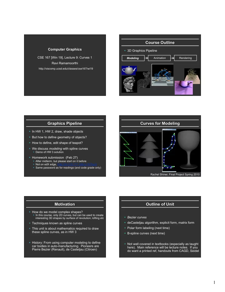
Course Outline Computer Graphics 3D Graphics Pipeline CSE 167 [Win 19], Lecture 9: Curves 1 Modeling Animation Rendering Ravi Ramamoorthi http://viscomp.ucsd.edu/classes/cse167/wi19 Graphics Pipeline Curves for Modeling In HW 1, HW 2,


slide-1
SLIDE 1

1

Computer Graphics

CSE 167 [Win 19], Lecture 9: Curves 1 Ravi Ramamoorthi

http://viscomp.ucsd.edu/classes/cse167/wi19

Course Outline

§ 3D Graphics Pipeline

Modeling Animation Rendering

Graphics Pipeline

§ In HW 1, HW 2, draw, shade objects § But how to define geometry of objects? § How to define, edit shape of teapot? § We discuss modeling with spline curves

§ Demo of HW 3 solution

§ Homework submission (Feb 27)

§ After midterm, but please start on it before § Not on edX edge, http://34.219.177.190/cs167hw3/ § Same password as for readings (and code grade only)

Curves for Modeling

Rachel Shiner, Final Project Spring 2010

Motivation

§ How do we model complex shapes?

§ In this course, only 2D curves, but can be used to create interesting 3D shapes by surface of revolution, lofting etc

§ Techniques known as spline curves § This unit is about mathematics required to draw these spline curves, as in HW 3 § History: From using computer modeling to define car bodies in auto-manufacturing. Pioneers are Pierre Bezier (Renault), de Casteljau (Citroen)

Outline of Unit

§ Bezier curves § deCasteljau algorithm, explicit form, matrix form § Polar form labeling (next time) § B-spline curves (next time) § Not well covered in textbooks (especially as taught here). Main reference will be lecture notes. If you do want a printed ref, handouts from CAGD, Seidel

slide-2
SLIDE 2

2

Bezier Curve (with HW3 demo)

§ Motivation: Draw a smooth intuitive curve (or surface) given few key user-specified control points

Demo HW 3

Control points (all that user specifies, edits) Smooth Bezier curve (drawn automatically) Control polygon

Bezier Curve: (Desirable) properties

§ Interpolates, is tangent to end points § Curve within convex hull of control polygon Control points (all that user specifies, edits) Smooth Bezier curve (drawn automatically) Control polygon

Survey

§ Anonymous, know how things are going § Will try to use it to improve course

Issues for Bezier Curves

Main question: Given control points and constraints (interpolation, tangent), how to construct curve? § Algorithmic: deCasteljau algorithm § Explicit: Bernstein-Bezier polynomial basis § 4x4 matrix for cubics § Properties: Advantages and Disadvantages

deCasteljau: Linear Bezier Curve

§ Just a simple linear combination or interpolation (easy to code up, very numerically stable)

Linear (Degree 1, Order 2)

F(0) = P0, F(1) = P1 F(u) = ? P0 P1 P0 P1 1-u u F(u) = (1-u) P0 + u P1 F(0) F(u) F(1)

deCasteljau: Quadratic Bezier Curve

P0 P1 P2 Quadratic Degree 2, Order 3 F(0) = P0, F(1) = P2 F(u) = ? F(u) = (1-u)2 P0 + 2u(1-u) P1 + u2 P2 P0 P1 P2 1-u 1-u u u 1-u u

slide-3
SLIDE 3

3

Geometric interpretation: Quadratic

u u u 1-u 1-u

Geometric Interpretation: Cubic

u u u u u u

deCasteljau: Cubic Bezier Curve

P0 P1 P2 P3 Cubic Degree 3, Order 4 F(0) = P0, F(1) = P3 P0 P1 P2 P3

1-u 1-u 1-u u u u u u u 1-u 1-u

F(u) = (1-u)3 P0 +3u(1-u)2 P1 +3u2(1-u) P2 + u3 P3

1-u

Summary: deCasteljau Algorithm

Linear Degree 1, Order 2 F(0) = P0, F(1) = P1

P0 P1 P0 P1 1-u u

F(u) = (1-u) P0 + u P1

P0 P1 P2

Quadratic Degree 2, Order 3 F(0) = P0, F(1) = P2

P0 P1 P2

F(u) = (1-u)2 P0 + 2u(1-u) P1 + u2 P2 1-u 1-u u u 1-u u

P0 P1 P2 P3

Cubic Degree 3, Order 4 F(0) = P0, F(1) = P3

P0 P1 P2 P3

1-u 1-u 1-u u u u u u u 1-u 1-u F(u) = (1-u)3 P0 +3u(1-u)2 P1 +3u2(1-u) P2 + u3 P3 1-u

DeCasteljau Implementation

§ Can be optimized to do without auxiliary storage

Summary of HW3 Implementation

Bezier (Bezier2 and Bspline discussed next time)

§ Arbitrary degree curve (number of control points) § Break curve into detail segments. Line segments for these § Evaluate curve at locations 0, 1/detail, 2/detail, … , 1 § Evaluation done using deCasteljau

§ Key implementation: deCasteljau for arbitrary degree

§ Is anyone confused? About handling arbitrary degree?

§ Can also use alternative formula if you want

§ Explicit Bernstein-Bezier polynomial form (next)

§ Questions?

slide-4
SLIDE 4

4

Issues for Bezier Curves

Main question: Given control points and constraints (interpolation, tangent), how to construct curve? § Algorithmic: deCasteljau algorithm § Explicit: Bernstein-Bezier polynomial basis § 4x4 matrix for cubics § Properties: Advantages and Disadvantages

Recap formulae

§ Linear combination of basis functions § Explicit form for basis functions? Guess it?

Linear: F(u) = P

0(1− u) + P 1u

Quadratic: F(u) = P

0(1− u)2 + P 1[2u(1− u)]+ P 2u2

Cubic: F(u) = P

0(1− u)3 + P 1[3u(1− u)2]+ P 2[3u2(1− u)]+ P 3u3

Degree n: F(u) = P

k k

Bk

n(u)

Bk

n(u) areBernstein-Bezier polynomials

Recap formulae

§ Linear combination of basis functions § Explicit form for basis functions? Guess it? § Binomial coefficients in [(1-u)+u]n

Linear: F(u) = P

0(1− u) + P 1u

Quadratic: F(u) = P

0(1− u)2 + P 1[2u(1− u)]+ P 2u2

Cubic: F(u) = P

0(1− u)3 + P 1[3u(1− u)2]+ P 2[3u2(1− u)]+ P 3u3

Degree n: F(u) = P

k k

Bk

n(u)

Bk

n(u) areBernstein-Bezier polynomials

Summary of Explicit Form

Bk

n(u) =

n! k!(n − k)!(1− u)n−kuk

Linear: F(u) = P

0(1− u) + P 1u

Quadratic: F(u) = P

0(1− u)2 + P 1[2u(1− u)]+ P 2u2

Cubic: F(u) = P

0(1− u)3 + P 1[3u(1− u)2]+ P 2[3u2(1− u)]+ P 3u3

Degree n: F(u) = P

k k

Bk

n(u)

Bk

n(u) areBernstein-Bezier polynomials

Issues for Bezier Curves

Main question: Given control points and constraints (interpolation, tangent), how to construct curve? § Algorithmic: deCasteljau algorithm § Explicit: Bernstein-Bezier polynomial basis § 4x4 matrix for cubics § Properties: Advantages and Disadvantages

Cubic 4x4 Matrix (derive)

F(u) = P

0(1− u)3 + P 1[3u(1− u)2]+ P 2[3u2(1− u)]+ P 3u3

= u3 u2 u 1

( )

M = ? ⎛ ⎝ ⎜ ⎜ ⎜ ⎜ ⎞ ⎠ ⎟ ⎟ ⎟ ⎟ P P

1

P

2

P

3

⎛ ⎝ ⎜ ⎜ ⎜ ⎜ ⎜ ⎞ ⎠ ⎟ ⎟ ⎟ ⎟ ⎟

slide-5
SLIDE 5

5

Cubic 4x4 Matrix (derive)

F(u) = P

0(1− u)3 + P 1[3u(1− u)2]+ P 2[3u2(1− u)]+ P 3u3

= u3 u2 u 1

( )

−1 3 −3 1 3 −6 3 −3 3 1 ⎛ ⎝ ⎜ ⎜ ⎜ ⎜ ⎞ ⎠ ⎟ ⎟ ⎟ ⎟ P P

1

P

2

P

3

⎛ ⎝ ⎜ ⎜ ⎜ ⎜ ⎜ ⎞ ⎠ ⎟ ⎟ ⎟ ⎟ ⎟

Issues for Bezier Curves

Main question: Given control points and constraints (interpolation, tangent), how to construct curve? § Algorithmic: deCasteljau algorithm § Explicit: Bernstein-Bezier polynomial basis § 4x4 matrix for cubics § Properties: Advantages and Disadvantages

Properties (brief discussion)

§ Demo of HW 3 § Interpolation: End-points, but approximates others § Single piece, moving one point affects whole curve (no local control as in B-splines later) § Invariant to translations, rotations, scales etc. That is, translating all control points translates entire curve § Easily subdivided into parts for drawing (next lecture): Hence, Bezier curves easiest for drawing