1 Mutation - selection equilibrium 1. Mutation pressure: ( ) ( ) - - PDF document

1

Population Genetics 7: transient verses equilibrium polymorphism

Mutation pressure and selection can operate in opposite directions as a force for change in allele frequencies in populations. Note that effectiveness of both depends on the allele frequency.

∆p is the change in allele frequency from one generation to the next. In this example, mutation and selection are acting in opposite directions as ∆p is positive under mutation pressure and negative under selection pressure. Note that the values of ∆p under both forces only become comparable when the allele frequency is low.

Frequency of a allele

µ = 0.0001

Mutation - selection equilibrium

∆p (mutation pressure) = ∆p (selection)

2

• 1. Mutation pressure:

Let µ = the mutation rate from A ⇒ a Let ν = the mutation rate from a ⇒ A Let pt = the frequency of A in the population in generation t. Let qt = the frequency of a in the population in generation t, with qt = (1 – pt).

( )

{

( )

{

ν µ

µ

rate at mutation by A to change that alleles a

• f

freq The rate at mutaion by a to change that alleles A

• f

freq The

v q p q − = ∆

Mutation - selection equilibrium

• 2. Natural selection against a deleterious recessive allele:

Remember form our earlier lecture: qt+1 = qt - sqt2 / 1- sqt2

So for ∆q, ∆q = qt+1 – qt ∆q = (qt - sqt2 / 1- sqt2) – qt ∆q = - sqt2(1- q) / 1- sqt2

Mutation - selection equilibrium

∆q (mutation pressure) = ∆q (selection) pµ - qν = sqt2(1- q) / 1- sqt2 YUCK! [Approximate and simplify] pµ = sqt2(1- q) / 1- sqt2 pµ = sqt2(1- q) (1-q)µ = sqt2(1- q) µ= sqt2 (approx.) [Dominance: q = µ/hs (approx.)]

3

Attainment of the equilibrium allele frequency given selection and a variety of different mutation rates. Note that the time to equilibrium varies in addition to the actual equilibrium frequencies.

s = 0.1 (Waa = 0.9) µ = mut rate A → a µ = 0.01 µ = 0.001 µ = 0.0001 µ = 0.00001

a Note that fore realistic mutation rates, the equilibrium frequencies are quite low (freq of a allele > 0.05). In this example selection pressure is also quite weak (s = 0.1). If we assume stronger selection pressure (s > 0.1), the equilibrium point will be lower and the rate to equilibrium will be faster.

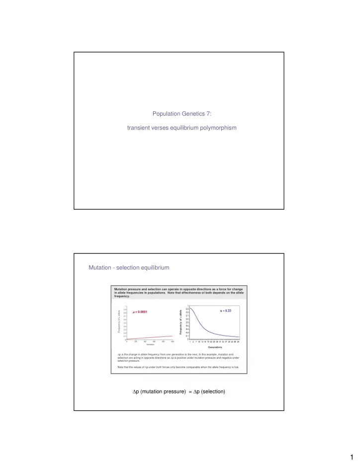
Mutation - selection equilibrium

Effect of partial dominance on mutation-selection equilibrium. The fitness of genotypes AA, Aa, and aa are assumed to be 1, 1–hs, and 1- s respectively.

0.005 0.01 0.015 0.02 0.025 0.03 0.035 0.000001 0.00001 0.0001 0.001 h = 0 h = 0.01 h = 0.05 h = 0.1 h = 0.5

Equilibrium frequency of recessive allele (a) Ratio of mutation rate to selection coefficient against aa (µ/s) The symbol h is the amount of dominance in the heterozygote genotype. Note, that even a small amount of dominance (h = 0.01) reduced the equilibrium frequency of the recessive

• allele. Hence, dominance has a significant influence on the equilibrium point. The reason

is that when q, the freq of the recessive allele is small, the majority of those alleles are in the heterozygote configuration, and even a small amount of selection on the heterozygotes leads to a major reduction in its equilibrium frequency as compared with full dominance. Note that for reasonable values of µ, h, and s, the equilibrium frequencies are < 0.01, This means that mutation selection equilibrium is not sufficient to explain low frequency detrimental alleles in populations where those alleles have frequencies > 0.01

Mutation - selection equilibrium

4

Selection - drift equilibrium

Drift alone: probability of fixation = 1/2Ne Selection + Drift: probability of fixation depends on interaction of s and Ne.

Nes > 1: beneficial allele more likely to be fixed than under drift alone Nes < 1: beneficial allele is fixed with probability close to its frequency in the population

Then fate of a beneficial recessive allele (A1) is not always predictable under the combined effects of directional selection and genetic drift. If there is no genetic drift (left: Nes = infinity), the fate of the recessive allele (A1) is always determined by selection. When there is drift (right: Nes < infinity) the fate of the recessive allele (A1) is not necessarily determined by selection; hence a deleterious allele can be fixed in a population. Nes = 100 Nes = infinity Note that Nes > 1 does not guarantee that an allele is going to be fixed, it simply indicates that (as a long term average) the frequency that it is fixed will be greater than the frequency under genetic drift alone.

Selection - drift

5

Selection - drift equilibrium

infinity 100 100 Nes 10% 0.01 0.1 Selection + Drift 1% 0.01 1 Drift alone 100% 0.01 0.1 Selection alone Fixation Initial frequency s System

s1 = 0.1 s2 = 0.3

Selection - drift

6

Because drift disturbs the allele frequencies each generation, frequencies in any one generation will not be in equilibrium. However, the long term average will be the equilibrium frequencies. The polymorphism in both of the above cases is not transient.

Equilibrium frequencies under balancing selection (s1 = 0.1 and s2 = 0.3) are less stable under the influence of genetic drift (right) as compared with an otherwise ideal population (left).

Selection - drift

Polymorphisms under balancing selection (s1 = 0.1 and s2 = 0.3) is transient if drift effects are strong. (Ne = 50).

Selection - drift

7

Combined effects of mutation, selection and drift on polymorphism. When drift is weak polymorphism is not transient, but when drift is strong the polymorphism is transient, but recurring due to mutation.

Nes = 100 Nes = 10 Nes = 1000 Nes = infinity

equilibrium

Mutation – selection – drift

Very high mutation rate (0.01) results in only a small shift in the long term average allele frequency under overdominant selection drift + selection µ = 0.01 Nes = 1000 drift + mutation + selection

Mutation – selection – drift

8

Mutation - drift equilibrium

• Ignored until 1960’s
• “Neutral theory of molecular evolution”
• Transient polymorphism
• Fundamental to discipline of molecular evolution

Sources of polymorphism in populations

• Mutation-selection-drift equilibrium (long-term or transient)
• Selection-drift (transient)
• Overdominance-drift equilibrium (long-term or transient)
• Mutation-drift (transient, but important)

9

• Drift constantly disturbs equilibrium.
• The strength of the disturbance depends on the effective population size (Ne).
• If strong enough, the disturbances can push the frequency to fixation.
• We don’t expect to see persistent equilibrium in populations with low Ne.
• For realistic values of µ, h and s, the equilibrium point is generally very low (p < 0.01).
• As an explanation for natural polymorphisms > 0.01, the balance between

mutation and selection is not satisfactory.

• Overdominance can explain population polymorphisms with frequencies > 0.01.
• A cost in fitness makes it unlikely that it can be invoked as a common mechanism

in natural populations.

• We will return the notion of the cost of selection later in this course.

Sources of polymorphism in populations