1 Classification by Control Structure Classification by Memory - - PDF document

SLIDE 1

1

Christoph Kessler, IDA, Linköpings universitet.

Introduction to Parallel Computing

Christoph Kessler

IDA, Linköping University

732A54 Big Data Analytics

2

• C. Kessler, IDA, Linköpings universitet.

Traditional Use of Parallel Computing: Large-Scale HPC Applications

NSC Triolith

High Performance Computing (HPC)

Much computational work (in FLOPs, floatingpoint operations) Often, large data sets E.g. climate simulations, particle physics, engineering, sequence

matching or proteine docking in bioinformatics, …

Single-CPU computers and even today’s

multicore processors cannot provide such massive computation power

Aggregate LOTS of computers Clusters

Need scalable parallel algorithms Need to exploit multiple levels of parallelism 3

• C. Kessler, IDA, Linköpings universitet.

More Recent Use of Parallel Computing: Big-Data Analytics Applications

Big Data Analytics

Data access intensive (disk I/O, memory accesses) Typically, very large data sets (GB … TB … PB … EB …) Also some computational work for combining/aggregating data E.g. data center applications, business analytics, click stream

analysis, scientific data analysis, machine learning, …

Soft real-time requirements on interactive querys

Single-CPU and multicore processors cannot

provide such massive computation power and I/O bandwidth+capacity

Aggregate LOTS of computers Clusters

Need scalable parallel algorithms Need to exploit multiple levels of parallelism Fault tolerance NSC Triolith 4

• C. Kessler, IDA, Linköpings universitet.

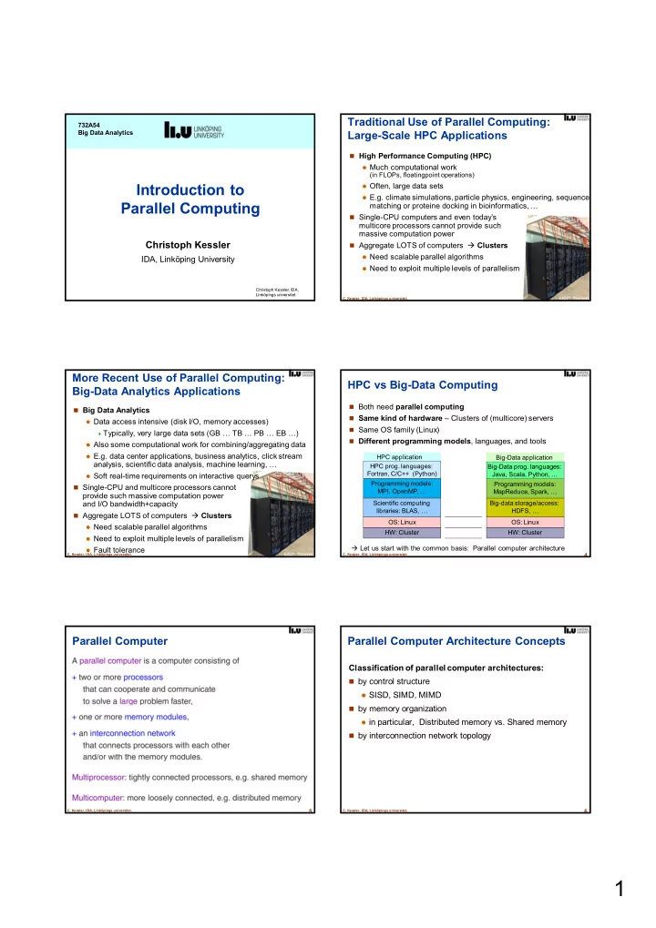
HPC vs Big-Data Computing

Both need parallel computing Same kind of hardware – Clusters of (multicore) servers Same OS family (Linux) Different programming models, languages, and tools HW: Cluster OS: Linux Programming models: MPI, OpenMP, … HW: Cluster OS: Linux Programming models: MapReduce, Spark, … HPC prog. languages: Fortran, C/C++ (Python) Big-Data prog. languages: Java, Scala, Python, … Let us start with the common basis: Parallel computer architecture Big-data storage/access: HDFS, … Scientific computing libraries: BLAS, … HPC application Big-Data application

5

• C. Kessler, IDA, Linköpings universitet.

Parallel Computer

6

• C. Kessler, IDA, Linköpings universitet.

Parallel Computer Architecture Concepts

Classification of parallel computer architectures:

by control structure

SISD, SIMD, MIMD

by memory organization

in particular, Distributed memory vs. Shared memory

by interconnection network topology

SLIDE 2

2

7

• C. Kessler, IDA, Linköpings universitet.

Classification by Control Structure

…

• p
• p
• p
• p
• p

1 2 3 4

8

• C. Kessler, IDA, Linköpings universitet.

Classification by Memory Organization

Most common today in HPC and Data centers:

Hybrid Memory System

• Cluster (distributed memory)
• f hundreds, thousands of

shared-memory servers each containing one or several multi-core CPUs

NSC Triolith

e.g. (traditional) HPC cluster e.g. multiprocessor (SMP) or computer with a standard multicoreCPU

9

• C. Kessler, IDA, Linköpings universitet.

Hybrid (Distributed + Shared) Memory

M M

10

• C. Kessler, IDA, Linköpings universitet.

Interconnection Networks (1)

Network

= physical interconnection medium (wires, switches) + communication protocol (a) connecting cluster nodes with each other (DMS) (b) connecting processors with memory modules (SMS) Classification

Direct / static interconnection networks

connecting nodes directly to each other Hardware routers (communication coprocessors)

can be used to offload processors from most communication work Switched / dynamic interconnection networks P R

11

• C. Kessler, IDA, Linköpings universitet.

Interconnection Networks (2): Simple Topologies

P P P P P P

fully connected 12

• C. Kessler, IDA, Linköpings universitet.

Interconnection Networks (3): Fat-Tree Network

Tree network extended for higher bandwidth (more switches,

more links) closer to the root

avoids bandwidth bottleneck

Example: Infiniband network (www.mellanox.com)

SLIDE 3

3

13

• C. Kessler, IDA, Linköpings universitet.

More about Interconnection Networks

Hypercube, Crossbar, Butterfly, Hybrid networks… TDDC78 Switching and routing algorithms Discussion of interconnection network properties

Cost (#switches, #lines) Scalability

(asymptotically, cost grows not much faster than #nodes)

Node degree Longest path ( latency) Accumulated bandwidth Fault tolerance (worst-case impact of node or switch failure) … 14

• C. Kessler, IDA, Linköpings universitet.

Example: Beowulf-class PC Clusters

with off-the-shelf CPUs (Xeon, Opteron, …)

15

• C. Kessler, IDA, Linköpings universitet.

Cluster Example: Triolith (NSC, 2012 / 2013)

A so-called Capability cluster (fast network for parallel applications, not for just lots of independent sequential jobs) 1200 HP SL230 servers (compute nodes), each equipped with 2 Intel E5-2660 (2.2 GHz Sandybridge) processors with 8 cores each 19200 cores in total Theoretical peak performance

• f 338 Tflops/s

Mellanox Infiniband network (Fat-tree topology)

NSC Triolith 16

• C. Kessler, IDA, Linköpings universitet.

The Challenge

Today, basically all computers are parallel computers!

Single-thread performance stagnating Dozens of cores and hundreds of HW threads available per server May even be heterogeneous (core types, accelerators) Data locality matters Large clusters for HPC and Data centers, require message passing

Utilizing more than one CPU core requires thread-level parallelism One of the biggest software challenges: Exploiting parallelism

Need LOTS of (mostly, independent) tasks to keep cores/HW threads

busy and overlap waiting times (cache misses, I/O accesses)

All application areas, not only traditional HPC

General-purpose, data mining, graphics, games, embedded, DSP, …

Affects HW/SW system architecture, programming languages,

algorithms, data structures …

Parallel programming is more error-prone

(deadlocks, races, further sources of inefficiencies)

And thus more expensive and time-consuming

17

• C. Kessler, IDA, Linköpings universitet.

Can’t the compiler fix it for us?

Automatic parallelization?

at compile time: Requires static analysis – not effective for pointer-based

languages

– inherently limited – missing runtime information needs programmer hints / rewriting ...

• k only for few benign special cases:

– loop vectorization – extraction of instruction-level parallelism

at run time (e.g. speculative multithreading) High overheads, not scalable

18

• C. Kessler, IDA, Linköpings universitet.

Insight

Design of efficient / scalable parallel algorithms is,

in general, a creative task that is not automatizable

But some good recipes exist …

Parallel algorithmic design patterns

SLIDE 4

4

19

• C. Kessler, IDA, Linköpings universitet.

The remaining solution …

Manual parallelization!

using a parallel programming language / framework, e.g. MPI message passing interface for distributed memory; Pthreads, OpenMP, TBB, … for shared-memory Generally harder, more error-prone than sequential

programming,

requires special programming expertise to exploit the HW

resources effectively

Promising approach:

Domain-specific languages/frameworks,

Restricted set of predefined constructs

doing most of the low-level stuff under the hood

e.g. MapReduce, Spark, … for big-data computing 20

• C. Kessler, IDA, Linköpings universitet.

Parallel Programming Model

System-software-enabled programmer’s view of the underlying hardware Abstracts from details of the underlying architecture, e.g. network topology Focuses on a few characteristic properties, e.g. memory model Portability of algorithms/programs across a family of parallel architectures Programmer’s view of the underlying system (Lang. constructs, API, …) Programming model Underlying parallel computer architecture

Mapping(s) performed by programming toolchain (compiler, runtime system, library, OS, …)

Shared Memory Message passing Christoph Kessler, IDA, Linköpings universitet.

Design and Analysis

• f Parallel Algorithms

Introduction

22

• C. Kessler, IDA, Linköpings universitet.

Foster’s Method for Design of Parallel Programs (”PCAM”)

PROBLEM + algorithmic approach PARTITIONING COMMUNICATION + SYNCHRONIZATION PARALLEL ALGORITHM DESIGN AGGLOMERATION PARALLEL ALGORITHM ENGINEERING

(Implementation and adaptation for a specific (type of) parallel computer)

Elementary Tasks

Textbook-style parallel algorithm

MAPPING + SCHEDULING

• I. Foster, Designing and Building Parallel Programs. Addison-Wesley, 1995.

P1 P2 P3

Macrotasks

23

• C. Kessler, IDA, Linköpings universitet.

Parallel Computation Model

= Programming Model + Cost Model

Christoph Kessler, IDA, Linköpings universitet.

Parallel Cost Models

A Quantitative Basis for the Design of Parallel Algorithms

SLIDE 5

5

25

• C. Kessler, IDA, Linköpings universitet.

Cost Model

26

• C. Kessler, IDA, Linköpings universitet.

How to analyze sequential algorithms:

The RAM (von Neumann) model for sequential computing

Basic operations (instructions):

• Arithmetic (add, mul, …) on registers
• Load
• Store
• Branch

Simplifyingassumptions for time analysis:

• All of these take 1 time unit
• Serial composition adds time costs

T(op1;op2) = T(op1)+T(op2)

• p
• p1
• p2

27

• C. Kessler, IDA, Linköpings universitet.

Analysis of sequential algorithms: RAM model (Random Access Machine)

s = d[0] for (i=1; i<N; i++) s = s + d[i] Data flow graph,

showing dependences (precedence constraints) between operations 28

• C. Kessler, IDA, Linköpings universitet.

The PRAM Model – a Parallel RAM

PRAM variants TDDD56, TDDC78 29

• C. Kessler, IDA, Linköpings universitet.

Remark

PRAM model is very idealized, extremely simplifying / abstracting from real parallel architectures: Good for early analysis of parallel algorithm designs: A parallel algorithm that does not scale under the PRAM model does not scale well anywhere else! The PRAM cost model has only 1 machine-specific parameter: the number of processors

30

• C. Kessler, IDA, Linköpings universitet.

A first parallel sum algorithm …

Data flow graph,

showing dependences (precedence constraints) between operations

Keep the sequential sum algorithm’s structure / data flow graph. Giving each processor one task (load, add) does not help much – All n loads could be done in parallel, but – Processor i needs to wait for partial result from processor i-1, for i=1,…,n-1 Still O(n) time steps! time

SLIDE 6

6

31

• C. Kessler, IDA, Linköpings universitet.

Divide&Conquer Parallel Sum Algorithm in the PRAM / Circuit (DAG) cost model

T(1) = O(1)

Recurrence equation for parallel execution time:

32

• C. Kessler, IDA, Linköpings universitet.

Divide&Conquer Parallel Sum Algorithm in the PRAM / Circuit (DAG) cost model

T(1) = O(1)

Recurrence equation for parallel execution time:

33

• C. Kessler, IDA, Linköpings universitet.

Recursive formulation of DC parallel sum algorithm in some programming model

cilk int parsum ( int *d, int from, int to ) { int mid, sumleft, sumright; if (from == to) return d[from]; // base case else { mid = (from + to) / 2; sumleft = spawn parsum ( d, from, mid ); sumright = parsum( d, mid+1, to ); sync; return sumleft + sumright; } } Implementation e.g. in Cilk: (shared memory) // The main program: main() { … parsum ( data, 0, n-1 ); … }

Fork-Join execution style: single task starts, tasks spawn child tasks for independent subtasks, and synchronize with them 34

• C. Kessler, IDA, Linköpings universitet.

Circuit / DAG model

Independent of how the parallel computation is expressed, the resulting (unfolded) task graph looks the same. Task graph is a directed acyclic graph (DAG) G=(V,E)

Set V of vertices: elementary tasks (taking time 1 resp. O(1) each) Set E of directed edges: dependences (partial order on tasks)

(v1,v2) in E v1 must be finished before v2 can start Critical path = longest path from an entry to an exit node

Length of critical path is a lower bound for parallel time complexity

Parallel time can be longer if number of processors is limited

schedule tasks to processors such that dependences are preserved

(by programmer (SPMD execution) or run-time system (fork-join exec.))

35

• C. Kessler, IDA, Linköpings universitet.

For a fixed number of processors … ?

Usually, p << n Requires scheduling the work to p processors

(A) manually, at algorithm design time:

Requires algorithm engineering E.g. stop the parallel divide-and-conquer e.g. at subproblem size n/p

and switch to sequential divide-and-conquer (= task agglomeration) For parallel sum:

Step 0. Partition the array of n elements in p slices of n/p

elements each (= domain decomposition)

Step 1. Each processor calculates a local sum for one slice,

using the sequential sum algorithm, resulting in p partial sums (intermediate values)

Step 2. The p processors run the parallel algorithm

to sum up the intermediate values to the global sum.

36

• C. Kessler, IDA, Linköpings universitet.

For a fixed number of processors … ?

Usually, p << n Requires scheduling the work to p processors

(B) automatically, at run time:

Requires a task-based runtime system

with dynamic scheduler

Each newly created task is dispatched

at runtime to an available worker processor.

Load balancing (overhead) Central task queue where idle workers

fetch next task to execute

Local task queues + Work stealing –

idle workers steal a task from some other processor

Run-time scheduler

…

Worker threads

1:1 pinned to cores

SLIDE 7

7

Christoph Kessler, IDA, Linköpings universitet.

Analysis of Parallel Algorithms

38

• C. Kessler, IDA, Linköpings universitet.

Analysis of Parallel Algorithms

Performance metrics of parallel programs

Parallel execution time

Counted from the start time of the earliest task

to the finishing time of the latest task

Work – the total number of performed elementary operations Cost – the product of parallel execution time and #processors Speed-up

the factor by how much faster we can solve a problem with p

processors than with 1 processor, usually in range (0…p)

Parallel efficiency = Speed-up / #processors, usually in (0…1) Throughput = #operations finished per second Scalability

does speedup keep growing well

also when #processors grows large?

High latency, high bandwidth

39

• C. Kessler, IDA, Linköpings universitet.

Analysis of Parallel Algorithms

Asymptotic Analysis

Estimation based on a cost model and algorithm idea

(pseudocode operations)

Discuss behavior for large problem sizes, large #processors

Empirical Analysis

Implement in a concrete parallel programming langauge Measure time on a concrete parallell computer

Vary number of processors used, as far as possible

More precise More work, and fixing bad designs at this stage is expensive

40

• C. Kessler, IDA, Linköpings universitet.

Parallel Time, Work, Cost

s = d[0] for (i=1; i<N;i++) s = s + d[i] 41

• C. Kessler, IDA, Linköpings universitet.

Parallel work, time, cost

>

42

• C. Kessler, IDA, Linköpings universitet.

Speedup

Speedup S(p) with p processors is usually in the range (0…p)

SLIDE 8

8

43

• C. Kessler, IDA, Linköpings universitet.

Amdahl’s Law: Upper bound on Speedup

44

• C. Kessler, IDA, Linköpings universitet.

Amdahl’s Law

45

• C. Kessler, IDA, Linköpings universitet.

Proof of Amdahl’s Law

Christoph Kessler, IDA, Linköpings universitet.

Towards More Realistic Cost Models

Modeling the cost of communication and data access

47

• C. Kessler, IDA, Linköpings universitet.

Modeling Communication Cost: Delay Model

48

• C. Kessler, IDA, Linköpings universitet.

core

Memory Hierarchy

And The Real Cost of Data Access

Processor / CPU cores

each containing few (~32) general-purpose data registers and L1 cache

L1 L2

L2 cache (on-chip) - ~1MB

L3

L3 cache (on-chip) – ~64MB Capacity [B] Transfer Block Size [B] Access Bandwidth [GB/s]

Primary Storage (DRAM)

Access Latency [ns] Very high Very fast (few cc) Very Slow (ms …s) Computer’s main memory (off-chip) ~64 GB

Secondary Storage (Hard Disk, SSD) I/O Network

(E.g. other nodes in a cluster; internet, …)

Cloud storage T ertiary Storage

(Tapes, …)

High (TB) Large (KB) Small (~10.. 100B) Small (~10KB) > 100 cc Mode- rate to low

SLIDE 9

9

49

• C. Kessler, IDA, Linköpings universitet.

Data Locality

Memory hierarchy rationale: Try to amortize the high access cost

• f lower levels (DRAM, disk, …) by caching data in higher levels for

faster subsequent accesses

Cache miss – stall the computation. fetch the block of data containing

the accessed address from next lower level, then resume

More reuse of cached data (cache hits) better performance

Working set = the set of memory addresses accessed together in

a period of computation

Data locality = property of a computation: keeping the working set

small during a computation

Temporal locality – re-access same data element multiple times

within a short time interval

Spatial locality – re-access neighbored memory addresses multiple

times within a short time interval High latency favors larger transfer block sizes (cache lines, memory

pages, file blocks, messages) for amortization over many subsequent accesses

50

• C. Kessler, IDA, Linköpings universitet.

Memory-bound vs. CPU-bound computation

Arithmetic intensity of a computation

= #arithmetic instructions (computational work) executed per accessed element of data in memory (after cache miss)

A computation is CPU-bound

if its arithmetic intensity is >> 1.

The performance bottleneck is the CPU’s arithmetic throughput

A computation is memory-access bound otherwise.

The performance bottleneck is memory accesses,

CPU is not fully utilized Examples:

Matrix-matrix-multiply (if properly implemented) is CPU-bound. Array global sum is memory-bound on most architectures.

Christoph Kessler, IDA, Linköpings universitet.

Some Parallel Algorithmic Design Patterns

52

• C. Kessler, IDA, Linköpings universitet.

Data Parallelism



Given:

One (or several) data containers x , z, … with n elements each,

e.g. array(s) x = (x1,...xn), z = (z1,…,zn), …

An operation f on individual elements of x, z, …

(e.g. incr, sqrt, mult, ...)



Compute: y = f(x) = ( f(x1), ..., f(xn) )



Parallelizability: Each data element defines a task

Fine grained parallelism Easily partitioned into independent tasks,

fits very well on all parallel architectures



Notation with higher-order function:

y = map ( f, x )

map(f,a,b):

53

• C. Kessler, IDA, Linköpings universitet.

Data-parallel Reduction



Given:

A data container x with n elements,

e.g. array x = (x1,...xn)

A binary, associative operation op on individual elements of x

(e.g. add, max, bitwise-or, ...)



Compute: y = OPi=1…n x = x1 op x2 op ... op xn



Parallelizability: Exploit associativity of op



Notation with higher-order function:

y = reduce ( op, x )

54

• C. Kessler, IDA, Linköpings universitet.

MapReduce (pattern)

A Map operation with operation f

• n one or several input data containers x, …,

producing a temporary output data container w, directly followed by a Reduce with operation g on w producing result y

y = MapReduce ( f, g, x, … ) Example:

Dot product of two vectors x, z: y = Σi xi * zi f = scalar multiplication, g = scalar addition

SLIDE 10

10

55

• C. Kessler, IDA, Linköpings universitet.

Task Farming



Independent subcomputations f1, f2, ..., fm could be done in parallel and/or in arbitrary

• rder, e.g.

independent loop iterations independent function calls 

Scheduling (mapping) problem

m tasks onto p processors static (before running) or dynamic Load balancing is important:

most loaded processor determines the parallel execution time



Notation with higher-order function:

farm (f1, ..., fm) (x1,...,xn)

f1 f2 P2 P1 P3 time

dispatcher f2 collector f1 fm …

56

• C. Kessler, IDA, Linköpings universitet.

Task Farming



Independent subcomputations f1, f2, ..., fm could be done in parallel and/or in arbitrary

• rder, e.g.

independent loop iterations independent function calls 

Scheduling (mapping) problem

m tasks onto p processors static (before running) or dynamic Load balancing is important:

most loaded processor determines the parallel execution time



Notation with higher-order function:

farm (f1, ..., fm) (x1,...,xn)

f1 f2 P2 P1 P3 time

dispatcher f2 collector f1 fm …

57

• C. Kessler, IDA, Linköpings universitet.

Parallel Divide-and-Conquer



(Sequential) Divide-and-conquer:

If given problem instance P is trivial, solve it directly. Otherwise: Divide: Decompose problem instance P in one or several smaller

independent instances of the same problem, P1, ..., Pk

For each i: solve Pi by recursion. Combine the solutions of the Pi into an overall solution for P 

Parallel Divide-and-Conquer:

Recursive calls can be done in parallel. Parallelize, if possible, also the divide and combine phase. Switch to sequential divide-and-conquer when enough parallel tasks

have been created.



Notation with higher-order function:

solution = DC ( divide, combine, istrivial, solvedirectly, n, P )

58

• C. Kessler, IDA, Linköpings universitet.

Example: Parallel Divide-and-Conquer

Example: Parallel Sum over integer-array x Exploit associativity: Sum(x1,...,xn) = Sum(x1,...xn/2) + Sum(xn/2+1,...,xn) Divide: trivial, split array x in place Combine is just an addition. y = DC ( split, add, nIsSmall, addFewInSeq, n, x ) Data parallel reductions are an important special case of DC.

59

• C. Kessler, IDA, Linköpings universitet.

Pipelining



applies a sequence of dependent computations/tasks (f1, f2, ..., fk) elementwise to data sequence x = (x1,x2,x3,...,xn)

For fixed xj, must compute fi(xj) before fi+1(xj) … and fi(xj) before fi(xj+1) if the tasks fi have a run-time state 

Parallelizability: Overlap execution of all fi for k subsequent xj

time=1: compute f1(x1) time=2: compute f1(x2) and f2(x1) time=3: compute f1(x3) and f2(x2) and f3(x1) ... Total time: O ( (n+k) maxi ( time(fi) )) with k processors Still, requires good mapping of the tasks fi to the processors

for even load balancing – often, static mapping (done before running)



Notation with higher-order function:

(y1,…,yn) = pipe ( (f1, ..., fk), (x1,…,xn) )

… x3 x2 x1 f1 f2 fk

60

• C. Kessler, IDA, Linköpings universitet.

Streaming

Streaming applies pipelining to processing

• f large (possibly, infinite) data streams

from or to memory, network or devices, usually partitioned in fixed-sized data packets,

in order to overlap the processing of

each packet of data in time with access of subsequent units of data and/or processing of preceding packets

• f data.

Examples

Video streaming from network to display Surveillance camera, face recognition Network data processing e.g. deep packet inspection … x3 x2 x1 f1 f2 f3

Read a packet of stream data Process a packet Process it more

fk

Write result

SLIDE 11

11

61

• C. Kessler, IDA, Linköpings universitet.

Stream Farming



Independent streaming subcomputations f1, f2, ..., fm

• n each data packet



Speed up the pipeline by parallel processing of subsequent data packets



In most cases, the original order of packets must be kept after processing dispatcher f2 collector f1 fm … … x3 x2 x1 … Combining streaming and task farming patterns

62

• C. Kessler, IDA, Linköpings universitet.

(Algorithmic) Skeletons



Skeletons are reusable, parameterizable SW components with well defined semantics for which efficient parallel implementations may be available.



Inspired by higher-order functions in functional programming



One or very few skeletons per parallel algorithmic paradigm

map, farm, DC, reduce, pipe, scan ... 

Parameterised in user code

• Customization by instantiating a skeleton template

in a user-provided function



Composition of skeleton instances in program code normally by sequencing+data flow

e.g. squaresum( x ) can be defined by

{ tmp = map( sqr, x ); return reduce( add, tmp ); } { mapreduce( sqr, add, x ) }

For frequent combinations, may define advanced skeletons, e.g.:

Image source:

• A. Ernstsson, 2016

63

• C. Kessler, IDA, Linköpings universitet.

SkePU

[Enmyren, K. 2010]

Skeleton programming library for heterogeneous multicore systems,

based on C++

Example: Global sum in SkePU-2 [Ernstsson 2016] Add

Add

Image source:

• A. Ernstsson, 2016

64

• C. Kessler, IDA, Linköpings universitet.

High-Level Parallel Programming with Skeletons

Skeletons (constructs) implement (parallel) algorithmic design patterns ☺ Abstraction, hiding complexity (parallelism and low-level programming) Enforces structuring, restricted set of constructs ☺ Parallelization for free ☺ Easier to analyze and transform Requires complete understanding and rewriting of a computation Available skeleton set does not always fit May lose some efficiency compared to manual parallelization Idea developed in HPC (mostly in Europe) since the late 1980s. Many (esp., academic) frameworks exist, mostly as libraries Industry (also beyond HPC domain) has adopted skeletons

map, reduce, scan in many modern parallel programming APIs e.g., Intel Threading Building Blocks (TBB): par. for, par. reduce, pipe NVIDIA Thrust Google MapReduce (for distributed data mining applications) 65

• C. Kessler, IDA, Linköpings universitet.

Further Reading

On PRAM model and Design and Analysis of Parallel Algorithms

• J. Keller, C. Kessler, J. Träff: Practical PRAM Programming. Wiley

Interscience, New York, 2001.

• J. JaJa: An introduction to parallel algorithms. Addison-Wesley, 1992.
• D. Cormen, C. Leiserson, R. Rivest: Introduction to Algorithms, Chapter
• 30. MIT press, 1989, or a later edition.
• H. Jordan, G. Alaghband: Fundamentals of Parallel Processing.

Prentice Hall, 2003.

• A. Grama, G. Karypis, V. Kumar, A. Gupta: Introduction to Parallel

Computing, 2nd Edition. Addison-Wesley, 2003. On skeleton programming, see e.g. our publications on SkePU: http://www.ida.liu.se/labs/pelab/skepu

66

• C. Kessler, IDA, Linköpings universitet.

Questions for Reflection

Model the overall cost of a streaming computation with a very large number N

• f input data elements on a single processor

(a) if implemented as a loop over the data elements running on an ordinary memory hierarchy with hardware caches (see above) (b) if overlapping computation for a data packet with transfer/access of the next data packet (b1) if the computation is CPU-bound (b2) if the computation is memory-bound Which property of streaming computations makes it possible to overlap computation with data transfer? Can each dataparallel computation be streamed? What are the performance advantages and disadvantages of large vs. small packet sizes in streaming? Why should servers in datacenters running I/O-intensive tasks (such as disk/DB accesses) get many more tasks to run than they have cores? How would you extend the skeleton programming approach for computations that operate on secondary storage (file/DB accesses)?