1 Markov Decision Processes Markov Decision Processes An MDP is - - PDF document

▶

Dec 18, 2022 265 likes •376 views

Non-Deterministic Search CSE 473: Artificial Intelligence Markov Decision Processes Dieter Fox University of Washington [Slides originally created by Dan Klein & Pieter Abbeel for CS188 Intro to AI at UC Berkeley. All CS188 materials are

SLIDE 1

CSE 473: Artificial Intelligence

Markov Decision Processes

Dieter Fox University of Washington

[Slides originally created by Dan Klein & Pieter Abbeel for CS188 Intro to AI at UC Berkeley. All CS188 materials are available at http://ai.berkeley.edu.]

Non-Deterministic Search Example: Grid World

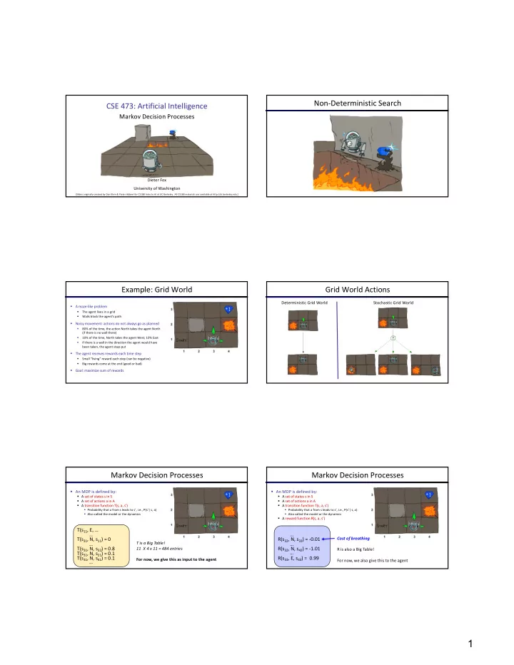
§ A maze-like problem

§ The agent lives in a grid § Walls block the agent’s path

§ Noisy movement: actions do not always go as planned

§ 80% of the time, the action North takes the agent North (if there is no wall there) § 10% of the time, North takes the agent West; 10% East § If there is a wall in the direction the agent would have been taken, the agent stays put

§ The agent receives rewards each time step

§ Small “living” reward each step (can be negative) § Big rewards come at the end (good or bad)

§ Goal: maximize sum of rewards

Grid World Actions

Deterministic Grid World Stochastic Grid World

Markov Decision Processes

§ An MDP is defined by:

§ A set of states s in S § A set of actions a in A § A transition function T(s, a, s’)

§ Probability that a from s leads to s’, i.e., P(s’| s, a) § Also called the model or the dynamics

T(s11, E, … … T(s31, N, s11) = 0 … T(s31, N, s32) = 0.8 T(s31, N, s21) = 0.1 T(s31, N, s41) = 0.1 …

T is a Big Table! 11 X 4 x 11 = 484 entries For now, we give this as input to the agent

Markov Decision Processes

§ An MDP is defined by:

§ A set of states s in S § A set of actions a in A § A transition function T(s, a, s’)

§ Probability that a from s leads to s’, i.e., P(s’| s, a) § Also called the model or the dynamics

§ A reward function R(s, a, s’)

… R(s32, N, s33) = -0.01 … R(s32, N, s42) = -1.01 R(s33, E, s43) = 0.99 …

Cost of breathing R is also a Big Table! For now, we also give this to the agent

SLIDE 2

Markov Decision Processes

§ An MDP is defined by:

§ A set of states s in S § A set of actions a in A § A transition function T(s, a, s’)

§ Probability that a from s leads to s’, i.e., P(s’| s, a) § Also called the model or the dynamics

§ A reward function R(s, a, s’)

§ Sometimes just R(s) or R(s’)

… R(s33) = -0.01 R(s42) = -1.01 R(s43) = 0.99

Markov Decision Processes

§ An MDP is defined by:

§ A set of states s in S § A set of actions a in A § A transition function T(s, a, s’)

§ Probability that a from s leads to s’, i.e., P(s’| s, a) § Also called the model or the dynamics

§ A reward function R(s, a, s’)

§ Sometimes just R(s) or R(s’)

§ A start state § Maybe a terminal state

§ MDPs are non-deterministic search problems

§ One way to solve them is with expectimax search § We’ll have a new tool soon

What is Markov about MDPs?

§ “Markov” generally means that given the present state, the future and the past are independent § For Markov decision processes, “Markov” means action

utcomes depend only on the current state

§ This is just like search, where the successor function could only depend on the current state (not the history)

Andrey Markov (1856-1922)

Policies

Optimal policy when R(s, a, s’) = -0.03 for all non-terminals s § In deterministic single-agent search problems, we wanted an optimal plan, or sequence of actions, from start to a goal § For MDPs, we want an optimal policy π*: S → A

§ A policy π gives an action for each state § An optimal policy is one that maximizes expected utility if followed § An explicit policy defines a reflex agent

§ Expectimax didn’t compute entire policies

§ It computed the action for a single state only

Optimal Policies

R(s) = -2.0 R(s) = -0.4 R(s) = -0.03 R(s) = -0.01

Example: Racing

SLIDE 3

Example: Racing

§ A robot car wants to travel far, quickly § Three states: Cool, Warm, Overheated § Two actions: Slow, Fast § Going faster gets double reward Cool Warm Overheated

Fast Fast Slow Slow 0.5 0.5 0.5 0.5 1.0 1.0 +1 +1 +1 +2 +2

Racing Search Tree MDP Search Trees

§ Each MDP state projects an expectimax-like search tree

a s s’ s, a (s,a,s’) called a transition T(s,a,s’) = P(s’|s,a) R(s,a,s’) s,a,s’ s is a state (s, a) is a q- state

Utilities of Sequences Utilities of Sequences

§ What preferences should an agent have over reward sequences? § More or less? § Now or later? [1, 2, 2] [2, 3, 4]

[0, 0, 1] [1, 0, 0]

Discounting

§ It’s reasonable to maximize the sum of rewards § It’s also reasonable to prefer rewards now to rewards later § One solution: values of rewards decay exponentially

Worth Now Worth Next Step Worth In Two Steps

SLIDE 4

Discounting

§ How to discount?

§ Each time we descend a level, we multiply in the discount once

§ Why discount?

§ Sooner rewards probably do have higher utility than later rewards § Also helps our algorithms converge

§ Example: discount of 0.5

§ U([1,2,3]) = 1*1 + 0.5*2 + 0.25*3 § U([1,2,3]) < U([3,2,1])

Stationary Preferences

§ Theorem: if we assume stationary preferences: § Then: there are only two ways to define utilities

§ Additive utility: § Discounted utility:

Quiz: Discounting

§ Given:

§ Actions: East, West, and Exit (only available in exit states a, e) § Transitions: deterministic

§ Quiz 1: For γ = 1, what is the optimal policy? § Quiz 2: For γ = 0.1, what is the optimal policy? § Quiz 3: For which γ are West and East equally good when in state d?

10*γ 3 = 1*γ γ 2 = 1 10

Infinite Utilities?!

§ Problem: What if the game lasts forever? Do we get infinite rewards? § Solutions:

§ Finite horizon: (similar to depth-limited search)

§ Terminate episodes after a fixed T steps (e.g. life) § Gives nonstationary policies (γ depends on time left)

§ Discounting: use 0 < γ < 1

§ Smaller γ means smaller “horizon” – shorter term focus

§ Absorbing state: guarantee that for every policy, a terminal state will eventually be reached (like “overheated” for racing)

Recap: Defining MDPs

§ Markov decision processes:

§ Set of states S § Start state s0 § Set of actions A § Transitions P(s’|s,a) (or T(s,a,s’)) § Rewards R(s,a,s’) (and discount γ)

§ MDP quantities so far:

§ Policy = Choice of action for each state § Utility = sum of (discounted) rewards

a s s, a s,a,s’ s’

Solving MDPs

§ Value Iteration § Policy Iteration § Reinforcement Learning

SLIDE 5

Optimal Quantities

§ The value (utility) of a state s: V*(s) = expected utility starting in s and acting optimally § The value (utility) of a q-state (s,a): Q*(s,a) = expected utility starting out having taken action a from state s and (thereafter) acting optimally § The optimal policy: π*(s) = optimal action from state s

a s s’ s, a

(s,a,s’) is a transition

s,a,s’

s is a state (s, a) is a q-state

Snapshot of Demo – Gridworld V Values

Noise = 0.2 Discount = 0.9 Living reward = 0

Snapshot of Demo – Gridworld Q Values

Noise = 0.2 Discount = 0.9 Living reward = 0

Values of States

§ Fundamental operation: compute the (expectimax) value of a state

§ Expected utility under optimal action § Average sum of (discounted) rewards § This is just what expectimax computed!

§ Recursive definition of value:

a s s, a s,a,s’ s’

Racing Search Tree Racing Search Tree

§ We’re doing way too much work with expectimax! § Problem: States are repeated

§ Idea: Only compute needed quantities once

§ Problem: Tree goes on forever

§ Idea: Do a depth-limited computation, but with increasing depths until change is small § Note: deep parts of the tree eventually don’t matter if γ < 1

SLIDE 6

Time-Limited Values

§ Key idea: time-limited values § Define Vk(s) to be the optimal value of s if the game ends in k more time steps

§ Equivalently, it’s what a depth-k expectimax would give from s

Computing Time-Limited Values Value Iteration The Bellman Equations

How to be optimal: Step 1: Take correct first action Step 2: Keep being optimal

The Bellman Equations

§ Definition of “optimal utility” via expectimax recurrence gives a simple one-step lookahead relationship amongst optimal utility values § These are the Bellman equations, and they characterize

ptimal values in a way we’ll use over and over

a s s, a s,a,s’ s’

Value Iteration

§ Bellman equations characterize the optimal values: § Value iteration computes them: § Value iteration is just a fixed point solution method

§ … though the Vk vectors are also interpretable as time-limited values

a V(s) s, a s,a,s’ V(s’)

SLIDE 7

Value Iteration Algorithm

§ Start with V0(s) = 0: § Given vector of Vk(s) values, do one ply of expectimax from each state: § Repeat until convergence § Complexity of each iteration: O(S2A) § Number of iterations: poly(|S|, |A|, 1/(1-γ)) § Theorem: will converge to unique optimal values

a Vk+1(s) s, a s,a,s’ ) s’ ( k V

k=0

Noise = 0.2 Discount = 0.9 Living reward = 0

k=1

Noise = 0.2 Discount = 0.9 Living reward = 0

k=2

Noise = 0.2 Discount = 0.9 Living reward = 0

k=3

Noise = 0.2 Discount = 0.9 Living reward = 0

k=4

Noise = 0.2 Discount = 0.9 Living reward = 0

SLIDE 8

k=5

Noise = 0.2 Discount = 0.9 Living reward = 0

k=6

Noise = 0.2 Discount = 0.9 Living reward = 0

k=7

Noise = 0.2 Discount = 0.9 Living reward = 0

k=8

Noise = 0.2 Discount = 0.9 Living reward = 0

k=9

Noise = 0.2 Discount = 0.9 Living reward = 0

k=10

Noise = 0.2 Discount = 0.9 Living reward = 0

SLIDE 9

k=11

Noise = 0.2 Discount = 0.9 Living reward = 0

k=12

Noise = 0.2 Discount = 0.9 Living reward = 0

k=100

Noise = 0.2 Discount = 0.9 Living reward = 0

Convergence*

§ How do we know the Vk vectors will converge? § Case 1: If the tree has maximum depth M, then VM holds the actual untruncated values § Case 2: If the discount is less than 1

§ Sketch: For any state Vk and Vk+1 can be viewed as depth k+1 expectimax results in nearly identical search trees § The max difference happens if big reward at k+1 level § That last layer is at best all RMAX § But everything is discounted by γk that far out § So Vk and Vk+1 are at most γk max|R| different § So as k increases, the values converge

Computing Actions from Values

§ Let’s imagine we have the optimal values V*(s) § How should we act?

§ It’s not obvious!

§ We need to do a mini-expectimax (one step) § This is called policy extraction, since it gets the policy implied by the values

Computing Actions from Q-Values

§ Let’s imagine we have the optimal q-values: § How should we act?

§ Completely trivial to decide!

§ Important lesson: actions are easier to select from q-values than values!

SLIDE 10

Problems with Value Iteration

§ Value iteration repeats the Bellman updates: § Problem 1: It’s slow – O(S2A) per iteration § Problem 2: The “max” at each state rarely changes § Problem 3: The policy often converges long before the values

a s s, a s,a,s’ s’

VI à Asynchronous VI

§ Is it essential to back up all states in each iteration?

§ No!

§ States may be backed up

§ many times or not at all § in any order

§ As long as no state gets starved…

§ convergence properties still hold!!

k=1

Noise = 0.2 Discount = 0.9 Living reward = 0

k=2

Noise = 0.2 Discount = 0.9 Living reward = 0

k=3

Noise = 0.2 Discount = 0.9 Living reward = 0

Asynch VI: Prioritized Sweeping

§ Why backup a state if values of successors same? § Prefer backing a state

§ whose successors had most change

§ Priority Queue of (state, expected change in value) § Backup in the order of priority § After backing a state update priority queue

§ for all predecessors