10/23/2015 CSE 473: Artificial Intelligence Autumn 2015 Hill - - PDF document

10/23/2015 1

CSE 473: Artificial Intelligence

Autumn 2015

1

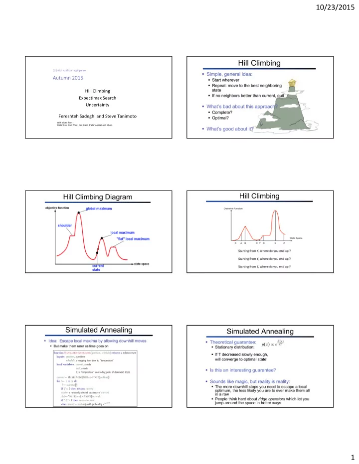
Hill Climbing Expectimax Search Uncertainty Fereshteh Sadeghi and Steve Tanimoto

With slides from : Dieter Fox, Dan Weld, Dan Klein, Pieter Abbeel and others.

10/23/2015 2

10/23/2015 3

Worst-Case vs. Average Case

10 10 9 100

max chance

Idea: Uncertain outcomes controlled by chance!

Probabilities Reminder: Probabilities

• A random variable represents an event whose outcome is unknown
• A probability distribution is an assignment of weights to outcomes
• Example: Traffic on freeway
• Random variable: T = whether there’s traffic
• Outcomes: T in {none, light, heavy}
• Distribution: P(T=none) = 0.25, P(T=light) = 0.50, P(T=heavy) = 0.25
• Some laws of probability (more later):
• Probabilities are always non-negative
• Probabilities over all possible outcomes sum to one
• As we get more evidence, probabilities may change:
• P(T=heavy) = 0.25,
• P(T=heavy | Hour=8am) = 0.60
• We’ll talk about methods for reasoning and updating probabilities later

0.25 0.50 0.25

• The expected value of a function of a random

variable is the average, weighted by the probability distribution over outcomes

• Example: How long to get to the airport?

Reminder: Expectations

0.25 0.50 0.25 Probability: 20 min 30 min 60 min Time:

35 min

x x x

+ +

10/23/2015 4

Worst-Case vs. Average Case

10 10 9 100

max min

Worst-Case vs. Average Case

10 10 9 100

max chance

Idea: Uncertain outcomes controlled by chance, not an adversary!

• In expectimax search, we have a

probabilistic model of how the opponent (or environment) will behave in any state

• Model could be a simple uniform distribution

(roll a die)

• Model could be sophisticated and require a

great deal of computation

• We have a chance node for any outcome out
• f our control: opponent or environment
• The model might say that adversarial actions

are likely!

• For now, assume each chance node

magically comes along with probabilities that specify the distribution over its

• utcomes

What Probabilities to Use? Randomness?

• Why wouldn’t we know the results of an

action?

• Explicit randomness: rolling dice
• Unpredictable opponents: the ghosts

respond erratically

• Actions can fail: when robot moves, its

wheels might slip

10 4 5 7

max chance

10 10 9 100

A1 A2

Expectimax Search

• Values now reflect average-case

(expected) outcomes, not worst-case (minimum) outcomes

• Expectimax search:

Compute average score under optimal play

• Max nodes as in minimax search
• Chance nodes are like min nodes but the
• utcome is uncertain. Calculate their

expected utilities

• I.e. take weighted average (expectation) of

children

10 4 5 7 10 10 9 100 [Demo: min vs exp (L7D1,2)]

max chance

Expectimax Pseudocode

def value(state): if the state is a terminal state: return the state’s utility if the next agent is MAX: return max-value(state) if the next agent is EXP: return exp-value(state) def exp-value(state): initialize v = 0 for each successor of state: p = probability(successor) v += p * value(successor) return v def max-value(state): initialize v = -∞ for each successor of state: v = max(v, value(successor)) return v

10/23/2015 5

Expectimax Pseudocode

def exp-value(state): initialize v = 0 for each successor of state: p = probability(successor) v += p * value(successor) return v

v = (1/2) (8) + (1/3) (24) + (1/6) (-12) = 5 7 8 24

• 12

1/2 1/3 1/6

10 10

Utilities Maximum Expected Utility

• Why should we average utilities?
• Principle of maximum expected utility:
• A rational agent should chose the action that

maximizes its expected utility, given its knowledge

• Questions:
• Where do utilities come from?
• How do we know such utilities even exist?
• How do we know that averaging even makes

sense?

• What if our behavior (preferences) can’t be

described by utilities?

Utilities

• Utilities are functions from
• utcomes (states of the world)

to real numbers that describe an agent’s preferences

• Where do utilities come from?
• In a game, may be simple (+1/-

1)

• Utilities summarize the agent’s

goals

• Theorem: any “rational”

preferences can be summarized as a utility function

• We hard-wire utilities and let

behaviors emerge

• Why don’t we let agents pick

utilities?

• Why don’t we prescribe

behaviors?

Utilities: Uncertain Outcomes

Getting ice cream Get Single Get Double Oops Whe w!

Preferences

• An agent must have preferences

among:

• Prizes: A, B, etc.
• Lotteries: situations with

uncertain prizes

• Notation:
• Preference:
• Indifference:

A B

p 1-p

A Lottery A Prize A

10/23/2015 6

Rationality

• We want some constraints on preferences before we call them rational,

such as:

• For example: an agent with intransitive preferences can

be induced to give away all of its money

• If B > C, then an agent with C would pay (say) 1 cent to get B
• If A > B, then an agent with B would pay (say) 1 cent to get A
• If C > A, then an agent with A would pay (say) 1 cent to get C

Rational Preferences

) ( ) ( ) ( C A C B B A     

Axiom of Transitivity:

Rational Preferences

Theorem: Rational preferences imply behavior describable as maximization of expected utility

The Axioms of Rationality

• Theorem [Ramsey, 1931; von Neumann & Morgenstern, 1944]
• Given any preferences satisfying these constraints, there exists a real-

valued function U such that:

• I.e. values assigned by U preserve preferences of both prizes and

lotteries!

• Maximum expected utility (MEU) principle:
• Choose the action that maximizes expected utility
• Note: an agent can be entirely rational (consistent with MEU) without

ever representing or manipulating utilities and probabilities

• E.g., a lookup table for perfect tic-tac-toe, a reflex vacuum cleaner

MEU Principle Human Utilities Human Utilities

Playing Russian Roulette?

10/23/2015 7

Playing Russian Roulette?

How much you would pay to avoid a a risk? What value people would place on their own lives?

Playing Russian Roulette?

How much you would pay to avoid a a risk? What value people would place on their own lives? Perhaps tens of thousands of dollars…??

Playing Russian Roulette?

How much you would pay to avoid a a risk? What value people would place on their own lives? Perhaps tens of thousands of dollars…??

micromort

Playing Russian Roulette?

How much you would pay to avoid a a risk? What value people would place on their own lives? Perhaps tens of thousands of dollars…??

micromort

The actual human behavior reflects a much lower monetary value for a micromort!!!

Playing Russian Roulette?

How much you would pay to avoid a a risk? What value people would place on their own lives? Perhaps tens of thousands of dollars…??

micromort

The actual human behavior reflects a much lower monetary value for a micromort!!! Driving for 230 miles incurs a risk of one micromort!! Over the life of your car (~92k miles) that’s 400 micromorts!! People are willing to pay $10k for a car that halves the risk of death!!

Utility Scales

• Normalized utilities: u+ = 1.0, u- = 0.0
• Micromorts: one-millionth chance of death,

useful for paying to reduce product risks, etc.

• QALYs: quality-adjusted life years, useful for

medical decisions involving substantial risk

• Note: behavior is invariant under positive linear

transformation

• With deterministic prizes only (no lottery

choices), only ordinal utility can be determined, i.e., total order on prizes

10/23/2015 8

Human Utilities

0.999999 0.000001

No change Pay $30 Instant death

• Utilities map states to real numbers. Which numbers?
• Standard approach to assessment (elicitation) of human

utilities:

• Compare a prize A to a standard lottery Lp between
• “best possible prize” u+ with probability p
• “worst possible catastrophe” u- with probability 1-p
• Adjust lottery probability p until indifference: A ~ Lp
• Resulting p is a utility in [0,1]

Utility of Money

• Money plays a significant rule in human utility functions
• Usually an agent prefers more money to less

Utility of Money

• Money plays a significant rule in human utility functions
• Usually an agent prefers more money to less
• The agent exhibits a monotonic preference for more money

Utility of Money

• Money plays a significant rule in human utility functions
• Usually an agent prefers more money to less
• The agent exhibits a monotonic preference for more money

But!

• This does not mean that money behaves as a utility function!
• This does not say anything about preferences between lotteries

involving money!

Money

• Money does not behave as a utility function, but we can

talk about the utility of having money (or being in debt)

• Given a lottery L = [p, $X; (1-p), $Y]
• The expected monetary value EMV(L) is p*X + (1-p)*Y
• U(L) = p*U($X) + (1-p)*U($Y)
• Typically, U(L) < U( EMV(L) )
• In this sense, people are risk-averse
• When deep in debt, people are risk-prone

Example:

• In a television game show:

A) take $1,000,000 prize B) gamble on the flip of a coin:

• If heads nothing
• If tails get $2,500,000

Which one you would take? A or B?

10/23/2015 9

Example:

• In a television game show:

A) take $1,000,000 prize B) gamble on the flip of a coin:

• If heads nothing
• If tails get $2,500,000
• If coin is fair, Expected Monetary Value (EMV) of gamble is:

EMV = ½ ($0) + ½ ($2,500,000) = $1,250,000  more than $1,000000

Example:

• In a television game show:

A) take $1,000,000 prize B) gamble on the flip of a coin:

• If heads nothing
• If tails get $2,500,000
• If coin is fair, Expected Monetary Value (EMV) of gamble is:

EMV = ½ ($0) + ½ ($2,500,000) = $1,250,000  more than $1,000000

Would you choose B?

Example:

• In a television game show:

A) take $1,000,000 prize B) gamble on the flip of a coin:

• If heads nothing
• If tails get $2,500,000
• If coin is fair, Expected Monetary Value (EMV) of gamble is:

EMV = ½ ($0) + ½ ($2,500,000) = $1,250,000 EU(B) = ½ U(Sk) + ½ U(Sk + $2,500,000) EU(A) = U(Sk + $1,000,000)

Example:

EMV = ½ ($0) + ½ ($2,500,000) = $1,250,000 EU(B) = ½ U(Sk) + ½ U(Sk + $2,500,000) EU(A) = U(Sk + $1,000,000) Utility is not directly proportional to monetary value Utility(first million) is very high! Utility(additional million) is smaller! U(Sk) = 5, U(Sk + $1,000,000) = 8 U(Sk + $2,500,000) = 9

Example:

EMV = ½ ($0) + ½ ($2,500,000) = $1,250,000 EU(B) = ½ U(Sk) + ½ U(Sk + $2,500,000) = 7 EU(A) = U(Sk + $1,000,000) = 8 Utility is not directly proportional to monetary value Utility(first million) is very high! Utility(additional million) is smaller! U(Sk) = 5, U(Sk + $1,000,000) = 8 U(Sk + $2,500,000) = 9

Example: Insurance

• Consider the lottery [0.5, $1000; 0.5,

$0]

• What is its expected monetary value?

($500)

• What is its certainty equivalent?
• Monetary value acceptable in lieu of

lottery

• $400 for most people
• Difference of $100 is the insurance

premium

• There’s an insurance industry because

people will pay to reduce their risk

• If everyone were risk-neutral, no insurance

needed!

• It’s win-win: you’d rather have the $400

and the insurance company would rather have the lottery (their utility curve is flat and they have many lotteries)

10/23/2015 10

Example: Human Rationality?

• Famous example of Allais (1953)
• A: [0.8, $4k; 0.2, $0]
• B: [1.0, $3k; 0.0, $0]
• C: [0.2, $4k; 0.8, $0]
• D: [0.25, $3k; 0.75, $0]
• Most people prefer B > A, C > D
• But if U($0) = 0, then
• B > A  U($3k) > 0.8 U($4k)
• C > D  0.8 U($4k) > U($3k)

Recommended

• Risks vs gains
• Probability estimates
• Cognitive architecture
• Much more

56