14 Symbolic MT 3: Phrase-based MT The previous two sections - - PDF document

SLIDE 1

14 Symbolic MT 3: Phrase-based MT

The previous two sections introduced word-by-word models of translation, how to learn them, and how to perform search with them. In this section, we’ll discuss expansions of this method to phrase-based machine translation (PBMT; [7]), which uses “phrases” of multiple sym- bols, which have allowed for highly effective models in a number of sequence-to-sequence tasks.

14.1 Advantages of Memorizing Multi-symbol Phrases

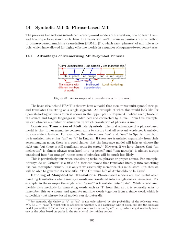
Comí un melocotón , una naranja y una manzana roja I ate a peach , an orange , and a red apple Translations with different numbers

• f words

Multi-word dependencies Local reorderings

Figure 41: An example of a translation with phrases. The basic idea behind PBMT is that we have a model that memorizes multi-symbol strings, and translates this string as a single segment. An example of what this would look like for Spanish-to-English translation is shown in the upper part of Figure 41, where each phrase in the source and target languages is underlined and connected by a line. From this example, we can observe a number of situations in which translation of phrases is useful: Consistent Translation of Multiple Symbols: The first advantage of a phrase-based model is that it can memorize coherent units to ensure that all relevant words get translated in a consistent fashion. For example, the determiners “un” and “una” in Spanish can both be translated into either “an” or “a” in English. If these are translated separately from their accompanying noun, there is a good chance that the language model will help us choose the right one, but there is still significant room for error.43 However, if we have phrases that “un melocot´

• n” is almost always translated into “a peach” and “una naranja” is almost always

translated into “an orange”, these sorts of mistakes will be much less likely. This is particularly true when translating technical phrases or proper names. For example, “Ensayo de un Crimen” is a title of a Mexican movie that translates literally into something like “an attempted crime”. It is only if we essentially memorize this multi-word unit that we will be able to generate its true title, “The Criminal Life of Archibaldo de la Cruz”. Handling of Many-to-One Translations: Phrase-based models are also useful when handling translations where multiple words are translated into a single one or vice-versa. For example, in the example the single word “comi´

• ” is translated into “I ate”. While word-based

models have methods for generating words such as “I” from thin air, it is generally safer to remember this as a chunk and generate multiple words together from a single word, which is something that phrase-based models can do naturally.

43For example, the choice of “a” or “an” is not only affected by the probability of the following word

P(et | et1 = “a/an00), which will be affected by whether et is a particular type of noun, but also the language model probability of “a” or “an” given the previous word P(et = “a/an00 | et1), which might randomly favor

• ne or the other based on quirks in the statistics of the training corpus.

106

SLIDE 2

Handling of Local Re-ordering Finally, in addition to getting the translations of words correct, it is necessary to ensure that they get translated in the proper order. Phrase-based models also have some capacity for short-distance re-ordering built directly into the model by memorizing chunks that contain reordered words. For example, in the phrase translating “una manzana roja” to “a red apple”, the order of “manazana/apple” and “roja/red” is reversed in the two languages. While this reordering between words can be modeled using an explicit reordering model (as described in Section 14.4), this can also be complicated and error

• prone. Thus, memorizing common reordered phrases can often be an effective for short-length

reordering phenomena.

14.2 A Monotonic Phrase-based Translation Model

So now that it’s clear that we would like to be modeling multi-word phrases, how do we express this in a formalized framework? First, we’ll tackle the simpler case where there is no explicit reordering, which is also called the case of monotonic transductions. In the previous section, we discussed an extremely simple monotonic model that modeled the noisy-channel translation model probability P(F | E) in a word-to-word fashion as follows: P(F | E) =

|E|

Y

t=1

P(ft | et). (138) To extend this model, we will first define ¯ F = f1, . . . , f| ¯

F| and ¯

E = e1, . . . , e| ¯

E|, which are

sequences of phrases. In the above example, this would mean that: ¯ F = {“com´ ı”, “un melocot´

• n”, . . . , “una manzana roja”}

(139) ¯ E = {“i ate”, “a peach”, . . . , “a red apple”}. (140) Given these equations, we would like to re-define our probability model P(F | E) with respect to these phrases. To do so, assume sequential process where we first translate tar- get words E into target phrases ¯ E, then translate target phrases ¯ E into source phrases ¯ F, then translate source phrases ¯ F into target words F. Assuming that all of these steps are independent, this can be expressed in the following equations: P(F, ¯ F, ¯ E | E) = P(F | ¯ F)P( ¯ F | ¯ E)P( ¯ E | E). (141) Starting from the easiest sub-model first, P(F | ¯ F) is trivial. This probability will be one whenever, the words in all the phrases of ¯ F can be concatenated together to form F, and zero

• therwise. To express this formally, we define the following function

F = concat( ¯ F). (142) The probability P( ¯ E | E), on the other hand is slightly less trivial. While E = concat( ¯ E) must hold, there are multiple possible segmentations ¯ E for any particular E, and thus this probability is not one. There are a number of ways of estimating this probability, the most common being either a constant probability for all segmentations: P( ¯ E | E) = 1 Z , (143) 107

SLIDE 3

• r a probability proportional to the number of phrases in the translation

P( ¯ E | E) = | ¯ E|λphrase-penalty Z . (144) Here Z is a normalization constant that ensures that the probability sums to one over all the possible segmentations. The latter method has a parameter λphrase-penalty, which has the intuitive effect of controlling whether we attempt to use fewer longer phrases λphrase-penalty < 0

• r more shorter phrases λphrase-penalty > 0. This penalty is often tuned as a parameter of the

model, as explained in detail in Section 14.6. Finally, the phrase translation model P( ¯ F | ¯ E) can is calculated in a way very similar to the word-based model, assuming that each phrase is independent: P( ¯ F | ¯ E) =

| ¯ E|

Y

t=1

P( ¯ ft | ¯ et). (145) This is conceptually simple, but it is necessary to be able to estimate the phrase translation probabilities P( ¯ ft | ¯ et) from data. We will describe this process in Section 14.3.

1 comí:<eps> 4 un:<eps> 8 ,:<eps> 10 una:<eps> 14 y:<eps> 2 <eps>:i 5 melocotón:<eps> 9 <eps>:, 11 naranja:<eps> 17 manzana:<eps> 15 <eps>:, 3 <eps>:ate

<eps>:<eps>/-log P_1

6 <eps>:a 7 <eps>:peach

<eps>:<eps>/-log P_2 <eps>:<eps>/-log P_3

12 <eps>:an 18 roja:<eps> 13 <eps>:orange

<eps>:<eps>/-log P_4

16 <eps>:and

<eps>:<eps>/-log P_5

19 <eps>:a 20 <eps>:red 21 <eps>:apple

<eps>:<eps>/-log P_6

Figure 42: An example of an WFST for a phrase-based translation model. log P n is an abbreviation for the negative log probability of the nth phrase, i.e., log P 1 is equal to P( ¯ f = “com´ ı” | ¯ e = “i ate”). But first, a quick note on how we would express a phrase-based translation model as a WFST. One of the nice things about the WFST framework is that this is actually quite simple; we simply create a path through the WFST that:

• 1. First reads in source words one at a time.
• 2. Then prints out the target words one at a time.
• 3. Finally, adds the log probability.

An example of this (using the phrases from Figure 41) is shown in Figure 42. This model can be essentially plugged in instead of the word-based translation model used in Section 13. 108

SLIDE 4

14.3 Phrase Extraction and Scoring

So now we have a translation model, how do we extract phrases from data and calculate their translation scores? Basically, the intuition behind the method is that we want to extract phrases that are consistent with word alignments, such as those obtained by the IBM models introduced in Section 12.

comí i a t e a r e d a p p l e una manzana roja comí → ate a → una manzana → apple roja → red comí una → ate a manzana roja → red apple comí una manzana roja→ ate a red apple comí → i ate comí una → i ate a comí una manzana roja→ i ate a red apple una manzana roja→ a red apple

Figure 43: Phrase extraction from aligned data. Phrases of various lengths (1: red, 2: blue, 3: yellow, 4: purple) are extracted. Phrases containing the null-aligned word “i” are extracted by appending it to neighboring phrases (green). An example of such alignments, and the phrases extracted from them, are shown in Fig- ure 43. In the example, we can note a few things. First, phrases of various lengths are extracted, from short phrases containing word-to-word alignments, and long phrases con- taining an entire sentence.44 This is important because it allows the translation system to remember and use longer phrases to improve its modeling accuracy, but also makes it possible to fall back to shorter phrases when necessary to maintain coverage. Phrases that contain words that are not aligned to any word in the counterpart language (null-aligned words; “i” in this example) are also included in phrases by connecting them to other phrases. This allows phrase-based models to generate these words in many-to-one translations, which is one

• f the advantages of phrase-based models mentioned above.

As a more formal definition of the phrases that we extract, if we have ei2

i1 containing the

i1th through i2th words of E, and f j2

j1 containing the j1th through j2th words of F, this will

be extracted as a phrases if and only if:

• There is at least one alignment link between the words in these phrases.
• The are no alignment links between words in ei2

i1 and f j11 1

• r f |F|

j2+1, and similarly no

alignment links between f j2

j1 and ei11 1

• r e|E|

i2+1.

The first restriction is to ensure that we don’t “hallucinate” phrases that contain no aligned

• words. The second restriction is to ensure that we don’t include phrases that have only part
• f the necessary content. An example of this would be f 4

2 e4 3 (“una manzana roja a

red”), which violates this restriction because f3 (“manzana”), which is included, is aligned to e4 (“apple”), which is not included.

44In interest of saving memory, it is common to limit the length of phrases to some number such as 5 or 7,

although there are methods around this limitation using efficient memory structures such as suffix trees [8].

109

SLIDE 5

A precise and efficient algorithm to extract these phrases (introduced in Figure 5.1 of [9]) is shown in Algorithm 6. Here, in Lines 2-3, we loop over all substrings in E. In Line 4, we declare a value TP (“target phrase”) which contains all positions in F that correspond to this substring ei2

• i1. In Line 5, we check if these values are quasi-consecutive, which means that

all the indices in the set are consecutive, with the exception of indices that are not aligned to any word in E. In Line 6-7, we calculate the span j1 to j2 in F. In Line 8 we calculate all positions in E that correspond to f j2

j1 , and in Line 9 we confirm that these indices indeed

fall between i1 and i2. Line 10 adds this phrase to the set of extracted phrase. The loop in Lines 11-18, and inner loop in Lines 13-16 respectively expand the source phrase f j2

j1 on the

left side and right side, adding unaligned words. Algorithm 6 The phrase extraction algorithm. Here A(i, j) indicates that ei is aligned to fj.

1: procedure PhraseExtract(E = e|E|

1 , F = f |F| 1 , A)

2:

for i1 from 1 to |E| do

3:

for i2 from i1 to |E| do

4:

TP := {j | 9i : i1  i  i2 ^ A(i, j)}

5:

if quasi-consecutive(TP) then

6:

j1 = min TP

7:

j2 = max TP

8:

SP := {i | 9j : j1  j  j2 ^ A(i, j)}

9:

if SP ⇢ {i1, i1 + 1, . . . , i2} then

10:

BP := BP [ {(ei2

i1, f j2 j1 }

11:

while j1 > 0 ^ 8i : A(i, j1) = 0 do

12:

j0 := j2

13:

while j0  J ^ 8i : A(i, j0) = 0 do

14:

BP := BP [ {(ei2

i1, f j0 j1}

15:

j0 := j0 + 1

16:

end while

17:

j1 := j1 1

18:

end while

19:

end if

20:

end if

21:

end for

22:

end forreturn BP

23: end procedure

This algorithm will extract many instances of phrases, resulting in a count c(f, e) of the number of times a particular phrase has been extracted. From these counts, we can directly calculate phrase translation probabilities P(f | e) that are used in Equation 145.

14.4 Phrase-based Translation with Reordering

It should be noted that the method described so far does not have any capacity for reordering

• f the phrases themselves. For many tasks, this reordering is not necessary, and even for tasks

110

SLIDE 6

where reordering is essential such as MT, it is possible to handle local word reorderings to some extent by memorizing local reorderings as parts of phrases (as mentioned in Section 14.1). In language pairs (such as English-Spanish, as noted by [1]), just handling this local reordering can get us pretty far.

kare wa momo to akai ringo wo tabeta he ate a peach and a red apple

Figure 44: An example of a phrase-based translation with inter-phrase reordering (for the phrase “wo tabeta/ate”. But for other language pairs with more disparate word order (e.g. German-English or Japanese-English) this is not sufficient. Thus, we would like to create a model that allows for examples that perform reordering of the phrases themselves, such as the Japanese-English example shown in Figure 44. In this example, we need to move the verb phrase “wo tabeta” at the end of the Japanese sentence to “ate” near the beginning of the English sentence. The basic idea of how we do this reordering is by relaxing the order with which we process the source phrases. We still generate the target sentence E in order, but do not necessarily translate the phrases in F sequentially, instead translating them in arbitrary order. This indi- cates that, like the IBM Models, we will have to have some concept of an “alignment” between phrases indicating which phrase translates into which. Thus, we re-structure Equation 145 as follows: P( ¯ F | ¯ E) =

| ¯ E|

Y

t=1

P( ¯ f¯

at) | ¯

etP(¯ at | ¯ at1

1

). (146) This indicates that we first select which phrase to translate next ¯ at, then calculate the prob- ability of its translation. The probability P(¯ at | ¯ at1

1

) is called the reordering model. The calculation of the reordering model is an area of active research, and there are quite a number of different methods [3, 4]. Of the various methods, the lexicalized reordering model of [11] is perhaps the most popular. The basic idea of this model is that based on the identity of the previous phrase h ¯ ft1, ¯ e¯

at1i, we want to estimate whether the reordering satisfies one of the following

patterns: Monotonic: No reordering occurs: ¯ at1 + 1 = ¯ at. Swap: A short-distance reordering that swaps the two phrases occurs: ¯ at1 1 = ¯ at. Discontinuous: Some other variety of reordering. These probabilities are generally estimated directly from data using maximum likelihood estimation. It should also be noted that we also need to keep track of the coverage of the phrases, so we will not select the same alignment twice in a single sentence, and thus P(at = i) = 0 if i has already been already used in a previous time step. 111

SLIDE 7

14.5 Search in Phrase-based Translation Models

kare wa momo to akai ringo wo tabeta E0 = C0 = E1 = he C1 = 1 1 E2 = he ate C2 = 1 1 E3 = he ate a peach C3 = E4 = he ate a peach and C4 = E5 = he ate a peach and a red apple C5 = 1 1 1 1 1 1 1 1 1 1 1 1 1 1 1 1 1 1 1 1 1 Figure 45: An example of the generation process for phrase-based MT. Now that we have a model that can handle reordering, we need to have an algorithm to generate translations. The generation process for the previous example is shown in Figure 45. Here, at each time step we have the target sentence at that point Et = concat(¯ et

1), and a

coverage vector, which is a binary vector Ct the same length as the source sentence, indicating which source words have been covered already by a phrase that we’ve used so far. This example is for a single translation E (and derivation D, expressing the phrases segmentation and alignment), but when actually generating translations it is necessary to be able to search over the space of all possible derivations. As we’ve seen in the previous sections, it is possible to perform search if we can create a WFST model that allows for this reordering. Unfortunately, it is not easy to create a general-purpose WFST that will do this reordering for all sentences. What we do instead is create a per-sentence expansion of all of the phrases as a search graph, which represents a WFST while not being strictly similar, similar to the search graph for neural MT systems shown in Section 7. An abbreviated example of such a search graph is shown in Figure 46. Each node represents a coverage vector, and each edge between nodes represents the translation of a particular phrase. The score of these edges would be the sum

• f the negative log phrase translation and reordering probabilities from Equation 146. Like

the word-based models in the previous section, this model can be composed with a WFST representing a language model, allowing for the full calculation of the conditional probability P(E | F). It should be noted that this search graph is extremely large. Even if we only consider

• ne-word phrases, and each word only has a single translation, just considering all the permu-

112

SLIDE 8

00000000 11000000 00100000 00010000 00000011

kare wa/he momo/ peach momo/ a peach to/and

...

wo tabeta/ate

...

11000011

wo tabeta/ ate

...

kare wa/he

11100000

momo/a peach

00001111

Input: kare wa momo to akai ringo wo tabeta akai ringo/ a red apple

Figure 46: An example of a search graph for phrase-based translation with reordering. For brevity weights are omitted from the edges, but these weight will be equal to log P( ¯ f|¯ e) for all phrase pairs. tations alone will result in an exponential number of combinations. In fact, it can be shown that translation with reordering in a word-based model with a 2-gram language model is an NP-hard problem [5], and thus we cannot reasonably expect to solve it exactly.45 As a result, we must resort to approximate search methods, such as the beam search that we used with neural MT models in subsubsection 7.2.3. The algorithm for phrase-based MT is basically the same as that used in neural MT, we step through the translation word-by-word, expand all our hypotheses, and keep only the best k. However, there is one slight complication: in phrase-based translation, there will be some phrases that consume a single word, and some phrases that consume multiple words, which means that even after we have expanded a single phrase, some of the hypotheses will be further along in their path towards the end of the sentence in Figure 46. To ensure that hypotheses that have progressed a similar amount are compared fairly, we use a multi-stack search algorithm, which maintains different “stacks” based on the number of covered words in the current partial hypothesis [12], and

• nly compares the scores of hypotheses within each of these stacks when deciding which

hypothesis to expand next.

14.6 A Log-linear Formulation for Translation

Finally, we will touch briefly upon an important extension that is widely used in symbolic translation models (among many other models in NLP): log-linear models [10]. To grasp the basic idea behind the log-linear models, first consider that in the following formulation we have four different models that participate in our translation: the language model P(E),

45Although with some tricks, it is possible to perform exact decoding for many, but not all sentences [2].

113

SLIDE 9

the phrase segmentation model P( ¯ E | E), the reordering model P(A | ¯ E),46 and the phrase translation model P( ¯ F | A, ¯ E). Normally these are multilpied together as P(F, D, E) = P( ¯ F | A, ¯ E)P(A | ¯ E)P( ¯ E | E)P(E), (147) where D includes the phrase segmentations ¯ F and ¯ E, as well as the alignment A. Equivalently, we can add together the log probabilities: log P(F, D, E) = log P( ¯ F | A, ¯ E) + log P(A | ¯ E) + log P( ¯ E | E) + log P(E). (148) The basic idea behind log-linear models is that we would like to generalize this equation by adding weights λ to each of these log-probabilities as follows:47 log P(F, D, E) / λTM log P( ¯ F | A, ¯ E) + λRM log P(A | ¯ E) + λSM log P( ¯ E | E) + λLM log P(E). (149) This allows us to modify the translation probability, giving relatively more weight to some of the component models. The motivation for this is two-fold. First, we would like to compensate for imperfections in modeling. While Equation 148 is exact, we have no guarantee that we will be able to accurately create each of these four component models and all models will all make modeling errors, some more egregious than others. By adding weights, we can decide which models we would like to trust more, and which models we would like to put less weight on, potentially increasing modeling accuracy. The second motivation is that this formulation actually allows us to add additional feature functions that would not fit into the framework easily if we had to deal strictly with conditional probabilities that we could multiply together sequentially like we have been doing previously. In fact, we can now generalize our equation to the following: log P(F, D, E) / X

i

λiφi(F, D, E), (150) where φi(·) is a feature function calculating some salient piece of information regarding the source and target sentences and the derivation. These features can, of course, include the log probabilities in Equation 149, but this framework also frees us to add additional feature functions that may be useful. For example, it is common to add: Word Penalty: A feature φWP(E) = |E|, which calculates the length of the target sentence. If λWP > 0, then the model will prefer longer sentences, and if λWP < 0 the model will prefer shorter sentences. Direct Translation Model: A feature that calculates not P( ¯ fat | ¯ et) for every phrase, but P(¯ et | ¯ fat). Considering the probabilities in both directions helps particularly in cases where ¯ et is relatively rare, and thus its conditional probability has been estimated from an insufficient amount of data.

46In actuality, parts of A may rely on previously selected phrases in ¯

F, but for simplicity here we ignore this fact.

47The symbol ∝ means “is proportional to”. In the case of log-linear models we would need to re-normalize

the value to get an actual probability distribution that sums to 1. However if our only purpose is to find the translation hypothesis with the best probability, we don’t need to worry about this normalization term.

114

SLIDE 10

Lexical Translation Model: Features, in both directions, that calculate the probability of phrases by the probabilities of their component words [6]. This can be helpful for longer phrases that themselves are rare and thus do not have well-estimated probabilities, but are composed of words whose probabilities are easier to estimate. Now, the only question is how we calculate the weights λ. One simple way to do so is using grid search, trying a bunch of values in a systematic fashion and seeing which one makes it possible to achieve the best translation accuracy. Of course, there are more sophisticated methods as well, which we will cover in detail in Section 18.

14.7 Exercise

In the exercise this time we will convert our monotonic word-based translation model from the previous section to a phrase-based model. This will entail two improvements:

• Implement the phrase extraction algorithm in Algorithm 6, and run it over the word

alignments obtained by your word alignment code from the exercise in Section 12.

• Implement code to convert this into a WFST.

The remainder will be very similar to what you did for the word-based models. One possible improvement includes implementing a log-linear model, which will allow you to introduce word or phrase penalties, or weight each component model of the phrase-based translation model. Implementing reordering within the model is another interesting, but potentially challenging extension.

References

[1] Francisco Casacuberta and Enrique Vidal. Machine translation with inferred stochastic finite-state

• transducers. Computational Linguistics, 30(2), 2004.

[2] Yin-Wen Chang and Michael Collins. Exact decoding of phrase-based translation models through lagrangian relaxation. In Proceedings of the 2011 Conference on Empirical Methods in Natural Language Processing (EMNLP), pages 26–37, 2011. [3] Michel Galley and Christopher D. Manning. A simple and effective hierarchical phrase reorder- ing model. In Proceedings of the 2008 Conference on Empirical Methods in Natural Language Processing (EMNLP), pages 848–856, 2008. [4] Isao Goto, Masao Utiyama, Eiichiro Sumita, Akihiro Tamura, and Sadao Kurohashi. Distortion model considering rich context for statistical machine translation. In Proceedings of the 51st Annual Meeting of the Association for Computational Linguistics (ACL), pages 155–165, 2013. [5] Kevin Knight. Decoding complexity in word-replacement translation models. Computational Linguistics, 25(4), 1999. [6] Philipp Koehn, Amittai Axelrod, Alexandra Birch Mayne, Chris Callison-Burch, Miles Osborne, and David Talbot. Edinburgh system description for the 2005 IWSLT speech translation eval- uation. In Proceedings of the 2005 International Workshop on Spoken Language Translation (IWSLT), 2005. [7] Phillip Koehn, Franz Josef Och, and Daniel Marcu. Statistical phrase-based translation. In Proceedings of the 2003 Human Language Technology Conference of the North American Chapter

• f the Association for Computational Linguistics (HLT-NAACL), pages 48–54, 2003.

115

SLIDE 11

[8] Adam Lopez. Hierarchical phrase-based translation with suffix arrays. In Proceedings of the 2007 Joint Conference on Empirical Methods in Natural Language Processing and Computational Natural Language Learning (EMNLP-CoNLL), pages 976–985, 2007. [9] Franz Josef Och. Statistical machine translation: from single-word models to alignment templates. PhD thesis, RWTH Aachen, 2002. [10] Franz Josef Och and Hermann Ney. Discriminative training and maximum entropy models for statistical machine translation. In Proceedings of the 40th Annual Meeting of the Association for Computational Linguistics (ACL), pages 295–302, 2002. [11] Christoph Tillman. A unigram orientation model for statistical machine translation. In Proceed- ings of the 2004 Human Language Technology Conference of the North American Chapter of the Association for Computational Linguistics (HLT-NAACL), pages 101–104, 2004. [12] Ye-Yi Wang and Alex Waibel. Decoding algorithm in statistical machine translation. In Proceed- ings of the 35th Annual Meeting of the Association for Computational Linguistics (ACL), pages 366–372, 1997.

116