19 Advanced Topics 1: MT System Combination In the chapters up to - - PDF document

19 Advanced Topics 1: MT System Combination

In the chapters up to this point, we have covered methods to create effective systems for machine translation. In actuality, when attempting to create the strongest possible system possible, it is common to combine together the results of multiple systems to create the best possible single translation possible. This method is called system combination or ensembling, and this chapter will cover the motivation and methods for doing so.

19.1 Why Combine Together Multiple Systems?

Before explicitly covering methods to perform system combination, it is worth thinking why we would want to do so in the first place. Obviously, creating two different machine translation systems (e.g. a phrase-based system and neural system) obviously takes more work than creating a single system in one of the two paradigms. However, there are in fact significant advantages to creating results with multiple systems and combining them together. In fact, there is a very intuitive argument for system combination: some systems are good at some things and other systems are good at other things. If we take a very simple method

• f training multiple systems and selecting which one to use in which situation, we should

be able to improve our results as a whole. For example, if we were creating a web-based translation system and we expected that users would often input short phrases in addition to full sentences, we might want to have a system based on looking up the short phrases in the dictionary, and then use the neural MT system if there was no hit in the dictionary. This is

• ne very simple variety of system combination.

Output 1: dog thinks

• f

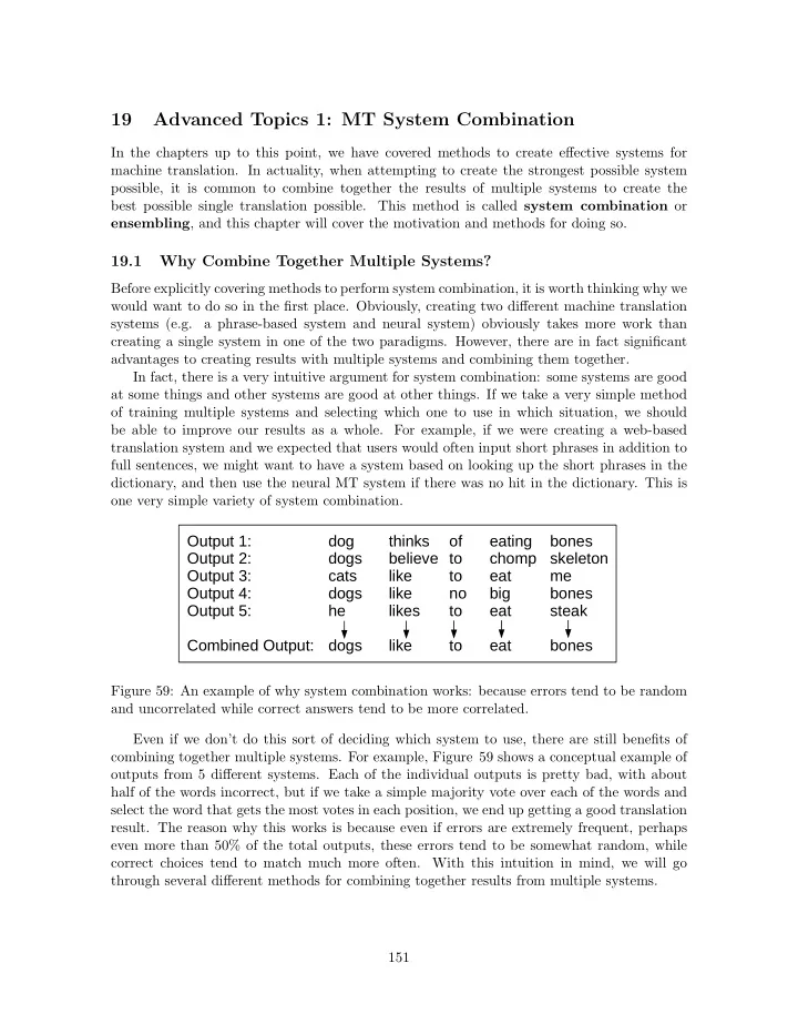
eating bones Output 2: dogs believe to chomp skeleton Output 3: cats like to eat me Output 4: dogs like no big bones Output 5: he likes to eat steak Combined Output: dogs like to eat bones

Figure 59: An example of why system combination works: because errors tend to be random and uncorrelated while correct answers tend to be more correlated. Even if we don’t do this sort of deciding which system to use, there are still benefits of combining together multiple systems. For example, Figure 59 shows a conceptual example of

• utputs from 5 different systems. Each of the individual outputs is pretty bad, with about

half of the words incorrect, but if we take a simple majority vote over each of the words and select the word that gets the most votes in each position, we end up getting a good translation

• result. The reason why this works is because even if errors are extremely frequent, perhaps

even more than 50% of the total outputs, these errors tend to be somewhat random, while correct choices tend to match much more often. With this intuition in mind, we will go through several different methods for combining together results from multiple systems. 151

19.2 Ensembling Decisions During Decoding

One simple but effective way of ensembling systems together that is widely used, particularly in neural machine translation systems, combines together the decisions predicted by multiple systems in the process of predicting the next word to output. Let’s say we have K neural machine translation systems, each of which can calculate a probability distribution of the next word given the input sentence and the previous words Pk(et | F, et−1

1

) (190) where Pk represents the probability distribution estimated by the kth system. This method takes in these K probability distributions and converts them into a new probability distri- bution P(et | F, et−1

1

), which is finally used when generating translations in the standard fashion. The simplest way that we can combine K probabilities into a single probability is linear interpolation, quite similar to the variety we used when combining together n-gram models with different orders P(et | F, et−1

1

) =

K

X

k=1

1 K Pk(et | F, et−1

1

). (191) This can also be parameterized so that the interpolation coefficient for each of the models is different P(et | F, et−1

1

) =

K

X

k=1

αkPk(et | F, et−1

1

) (192) under the restriction that all values of αk are between 0 and 1 and add to 1 in order to assure that we have a well-formed probability distribution. It is also possible to perform log-linear interpolation, where we add together the prob- abilities of each model in log space, then perform a softmax to get the final probability: P(et | F, et−1

1

) = softmax(

K

X

k=1

αk log Pk(et | F, et−1

1

)). (193) Here it is necessary to normalize the probabilities with the softmax after combining them together, as the sum of the log probabilities won’t necessarily result in a well-formed log probability distribution, and thus we need to re-normalize to ensure that the distribution is

• correct. As a result of this, the values of αk do not necessarily need to add to 1, and can take

any values we choose. These methods have a very similar form, but the results are quite different. Specifically, linear interpolation will tend to favor hypotheses where any one of the models assigns a high score (similar to the logical “or”), while log-linear interpolation will favor hypotheses where all of the models agree (similar to the logical “and”).57 Thus, when we prefer that all models are able to confirm a solution, we use log-linear interpolation, and when we prefer that models both propose complimentary solutions, we use linear interpolation.

57Question: Confirm this by noting that happens with each method when calculating the ensembled probability

• f three events when the probabilities according to model one are {0.6, 0.3, 0.1} and according to model two are

{0.05, 0.3, 0.65}.

152

19.3 Post-hoc System Combination

The method in the previous section is based on combining together multiple models that make decisions about the next word in the sentnece, like neural models. However, let’s say we want to combine together very different models that make predictions in very different ways, such as a neural model, a phrase-based model, and a tree-based model. In this case, it is common to first generate hypotheses with each of these different models, then use these inde- pendently generated hypotheses to select the best possible solution. Within this framework, there are generally two different ways to combine together hypotheses from different systems: reranking and generative combination. 19.3.1 Reranking-based Combination Reranking consists of taking the hypotheses generated by each system, and using some mea- sure of their goodness to select the best one. One simple example of reranking would be to generate N hypotheses for each of the K systems, then select the best of these hypotheses according to the overall probability calculated by each of the systems. More formally, we calculate a sample of N hypotheses for each system k: Ek = N − max

E

Pk(E | F). (194) Then we decide the overall space of hypotheses that we will consider as the union of all hypotheses generated by each system E =

K

[

k=1

Ek. (195) We define the probability of each hypothesis P(E | F) as the linear (Equation 192) or log- linear (Equation 193) interpolation of the model probabilities, and then select the hypothesis that has the highest probability according to these interpolated probabilities ˆ E = argmax

E∈E

P(E | F). (196) 19.3.2 Minimum Bayes Risk One other widely used criterion for choosing hypotheses that is simple yet effective in both single-system and multi-system reranking is the minimum Bayes risk decision criterion [6]. From the minimum risk training in Section 18.3, we can remember that risk is defined as the expected error of a particular hypothesis E risk(E, F) = X

˜ E

P( ˜ E | F)error(E, ˜ E). (197) In contrast to simply taking the hypothesis with the highest posterior probability in Equa- tion 196 (the max a posteriori (MAP) decision rule) minimum Bayes risk decision rule is an alternative that attempts to minimize this risk ˆ E = argmin

E∈E

risk(E, F). (198) 153

# Translation P(E | F) E1 this is an example 0.4 E2 this is an example of minimum Bayes risk 0.2 E3 this was an example of minimum Bayes risk 0.25 E4 this is minimum Bayes risk 0.1 BLEU+1 given ref E[BLEU+1] risk E1 E2 E3 E4 E1 1.0 0.37 0.18 0.35 0.57 0.43 E2 0.43 1.0 0.75 0.35 0.61 0.39 E3 0.22 0.75 1.0 0.31 0.53 0.47 E4 0.34 0.33 0.29 1.0 0.42 0.58 Table 1: An example of the difference between choosing a hypothesis based on probability and based on risk. A practical example of the consequences of this decision rule is shown in Table 1. In this example, we can see that the first sentence E1 gets significantly higher probability than any

• f the other hypotheses. However, E2 is the most similar hypothesis to the other hypotheses

in the space, as indicated by its relatively high BLEU scores when using the other sentences in the n-best list as a reference. as a result, when we take the expectation of the BLEU score, we can find that the expected BLEU of E2 is higher than E1 and E3 which have higher probabilities, but are more different from the other hypotheses in the space of hypotheses that we are considering. By taking into account this similarity, we are able to pick hypotheses that are more likely to be correct with respect to the other hypotheses, which helps us avoid picking hypotheses that might have high probability, but would be really bad mistakes if one

• f the other hypotheses was actually the correct one.

19.3.3 Tunable Combination It is also possible to treat system combination as a problem of doing machine translation all

• ver again, starting with the hypotheses generated by the systems that we want to combine.

For example, it is possible to to combine together multiple lattices of translation results into a single search lattice, then use search methods from phrase-based translation to find the best hypothesis [8, 2]. This method is able to generate new hypotheses that are not explicitly included in the n-best or lattice results of any individual system, and can also take advantage

• f the ability of phrase-based systems to be tuned to maximize BLEU score or incorporate

large language models, etc.

19.4 Desiderata for System to be Combined

The previous couple sections have said “let’s assume that we have K systems” and described methods to combine them together. However, this also leaves open the natural question about exactly which kinds of systems we should be creating in order to combine them together. The following are several rules of thumb that can be useful when creating these systems: Favor Quality The biggest rule of thumb is one that is relatively obvious: the systems that 154

we are combining should be good systems in the first place. They should also be of relatively uniform quality, as if there is a single system that is much better than the rest, it is possible that the combined system will not be able to exceed the accuracy of the single-best system, or may even be dragged down by the others. Favor Diversity Another favorable quality is diversity; it is often better that the systems going into the combination method are of different types. For example, we may want to use one neural system, one phrase-based system, and one tree-based system. The reason for this stems from the fact that, as stated in Section 19.1, it is important for errors to be uncorrelated. In general, systems using different paradigms will make very different mistakes, decreasing the correlation between errors, and increasing the post-combination performance. That being said, even training multiple neural systems with exactly the same architecture but different random seeds still provides a significant boost in performance. Favor Quantity Finally, where possible it is best to have a large number of models in the

• ensemble. The main downside to this is that it becomes necessary to train multiple

models, and at test time it is necessary to calculate according to all of these models. This generally makes computation increase linearly in the size of the ensemble.

19.5 Ensemble Distillation

The ensembling methods described in this chapter are quite effective, frustratingly so at times, to the point where they are an essential tool to practicioners who must get the highest possible accuracy on a particular task. However, ensembles also come at a large cost, both at training time when we have to train multiple models, and at test time when we have to make predictions with each of the models, which requires K times more memory and computation time than prediction with a single model. One way to alleviate this problem is through model distillation or teacher-student methods, a process of training a new model based on the predictions of K models [3, 5]. One simple way to do so that has been effective in the context of neural network classification models is based on training an teacher ensemble of models to predict a probability distribution: Pt(y|x) =

K

X

k=1

Pk(y|x), (199) and then creating another student network that attempts to learn to make its probability Ps(x) copy this teacher distribution. Specifically, we can define the loss function to train the student network to be the cross-entropy of the teacher distribution given the student distribution as follows: H(y, x, Pt, Ps) = − X

˜ y

Pt(˜ y|x) log Ps(˜ y|x). (200) If we assume that the teacher network is always correct, assigning probability of 1 to the correct answer and 0 to everything else, this reduces to the standard negative log-likelihood

• bjective that we usually use when training neural networks.

155

When applying these methods to sequence-generation problems, things are a bit more

• difficult. We could think of a sequence-level distillation objective such as the following:

H(E, F, Pt, Ps) = − X

˜ E

Pt( ˜ E|F) log Ps( ˜ E|F), (201) but this requires enumerating over all the possible sentences in the target language, and is thus not practical. [5] describe a number of alternative methods: Word-level Calculation: In this method, we calculate the entropy on a word-by-word-basis H(E, F, Pt, Ps) ≈ −

|E|

X

t=1

X

˜ et

Pt(˜ et|F, et−1

1

) log Ps(˜ et|F, et−1

1

). (202) Sampling-based Approximation: In this method, we simply sample a sentence from the teacher distribution, and optimize the student distribution using maximum likelihood with this sampled sentence as the ground truth. This is similar to the self-training mentioned in Section 18.6, and will get the student network to try to create hypotheses that match the distribution of the teacher. Finally, one simple and practical way to combine multiple models (with the same parame- ter space) into a single model is parameter averaging [1, 4]. In this method we simply take the parameters θk of our K models and average them together to get our final parameter set: θ = 1 K

K

X

k=1

θk. (203) This method is efficient and easy to implement, as it does not require any extra training. However, in neural networks with hidden layers, because each node in the hidden layer might represent a different feature in each training run, simply averaging together the parameters does not result in a coherent model, and accuracy will plummet. However, within a single training run, and particularly at the end of training, we can expect that the parameters will not make large changes in the space and the semantics of the nodes in the hidden layer of the model will be similar. Thus, it is possible to save the parameters periodically several times near the end of the training process, then average them together at the end. [4] and others have reported that this stabilizes training for neural machine translation without the costly process of training multiple models.

19.6 Further Reading

Theoretical Guarantees and Boosting: [7] shows that if we combine together multiple weak learners, which are only able to perform the classification task at a rate slightly better than chance, it is possible (with a few conditions) to create a strong learner that is able to perform arbitrarily well on the data. This is interesting in that it provides some theoretical grounding for why system combination works so well, and also because it led to the boosting algorithm, where learners are trained on examples where previous learners failed to perform well. Similar concepts have been used (within a single-system context) to improve the training of neural MT systems [9]. 156

19.7 Exercise

As an exercise, you could implement ensembling for your neural machine translation system. This would entail the following:

• 1. Training multiple neural machine translation systems using different random seeds. Al-

ternatively, you could train models with different structures or on different subsets of the data.

• 2. Modifying your search code to make it possible to read in multiple models and calculate

the linear or log-linear combination of their probability distributions while generating hypotheses.

• 3. Generate hypotheses with this ensembled model and measure the accuracy.

References

[1] Michael Collins. Discriminative training methods for hidden Markov models: Theory and exper- iments with perceptron algorithms. In Proceedings of the Conference on Empirical Methods in Natural Language Processing (EMNLP), pages 1–8, 2002. [2] Kenneth Heafield and Alon Lavie. Combining machine translation output with open source: The carnegie mellon multi-engine machine translation scheme. The Prague Bulletin of Mathematical Linguistics, 93:27–36, 2010. [3] Geoffrey Hinton, Oriol Vinyals, and Jeff Dean. Distilling the knowledge in a neural network. arXiv preprint arXiv:1503.02531, 2015. [4] Marcin Junczys-Dowmunt, Tomasz Dwojak, and Rico Sennrich. The amu-uedin submission to the wmt16 news translation task: Attention-based nmt models as feature functions in phrase-based

• smt. arXiv preprint arXiv:1605.04809, 2016.

[5] Yoon Kim and Alexander M Rush. Sequence-level knowledge distillation. arXiv preprint arXiv:1606.07947, 2016. [6] Shankar Kumar and William Byrne. Minimum Bayes-risk decoding for statistical machine trans-

• lation. In Proceedings of the 2004 Human Language Technology Conference of the North American

Chapter of the Association for Computational Linguistics (HLT-NAACL), 2004. [7] Robert E Schapire. The strength of weak learnability. Machine learning, 5(2):197–227, 1990. [8] Khe Chai Sim, William J Byrne, Mark JF Gales, Hichem Sahbi, and Philip C Woodland. Consensus network decoding for statistical machine translation system combination. In Acoustics, Speech and Signal Processing, 2007. ICASSP 2007. IEEE International Conference on, volume 4, pages IV–

• 105. IEEE, 2007.

[9] Dakun Zhang, Jungi Kim, Josep Crego, and Jean Senellart. Boosting neural machine translation. arXiv preprint arXiv:1612.06138, 2016.

157