2.4 Partitioned Matrices In real world problems, systems can have - - PDF document

2.4 Partitioned Matrices

In real world problems, systems can have huge numbers of equations and un-

• knowns. Thousands of equations and hundreds of thousands of variables are not
• uncommon. Standard computation techniques are inefficient in such cases, so we

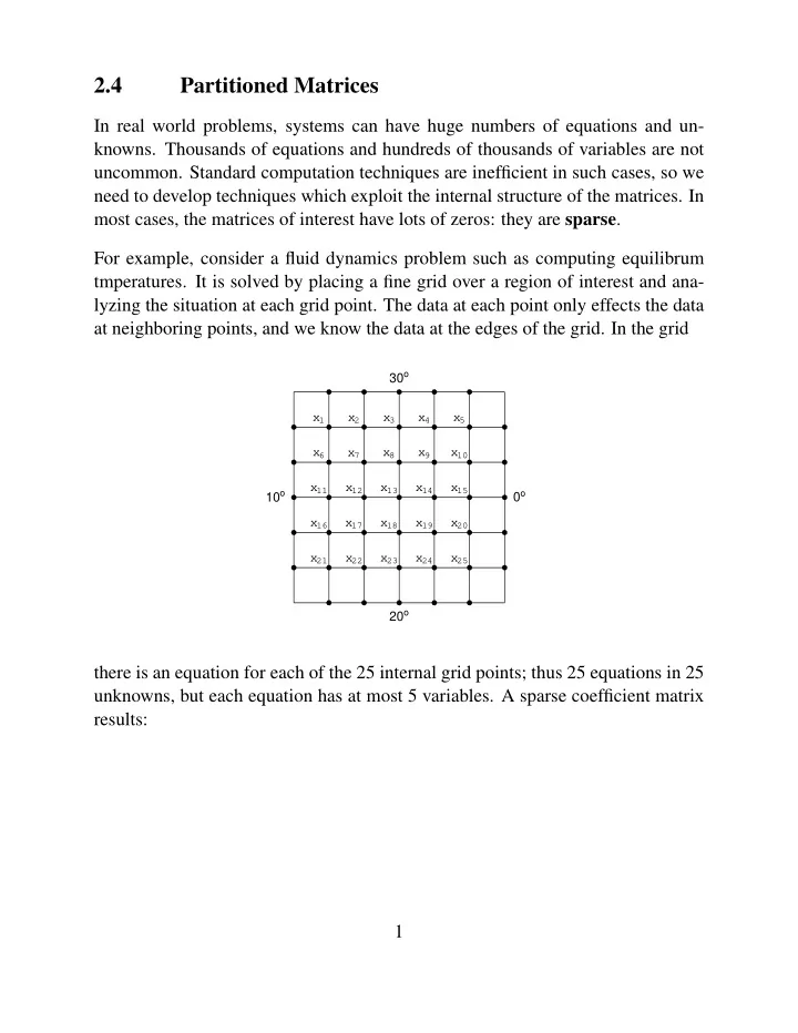
need to develop techniques which exploit the internal structure of the matrices. In most cases, the matrices of interest have lots of zeros: they are sparse. For example, consider a fluid dynamics problem such as computing equilibrum

• tmperatures. It is solved by placing a fine grid over a region of interest and ana-

lyzing the situation at each grid point. The data at each point only effects the data at neighboring points, and we know the data at the edges of the grid. In the grid

10o 0o 20o 30o x1 x2 x3 x4 x5 x6 x7 x8 x9 x10 x11 x12 x13 x14 x15 x16 x17 x18 x19 x20 x21 x22 x23 x24 x25

there is an equation for each of the 25 internal grid points; thus 25 equations in 25 unknowns, but each equation has at most 5 variables. A sparse coefficient matrix results: 1

2                       

• 

                      Partitioning a matrix: Splitting it up into smaller matrices. Consider A =     2 1 −3 5 7 1 4 −1 2 3 −2 1 1 5 4 1 −3     Example 1: One way to partition A:     2 1 −3 5 7 1 4 −1 2 3 −2 1 1 5 4 1 −3     which is recorded A11 = 2 1 0 1

• , A12 =

−3 5 7 4 −1 2

• A21 =

3 −2 4

• , A22 =

1 1 5 0 1 −3

3 Example 2: Another way to partition A:     2 1 −3 5 7 1 4 −1 2 3 −2 1 1 5 4 1 −3     Example 3: Another way to partition A:     2 1 −3 5 7 1 4 −1 2 3 −2 1 1 5 4 1 −3     Example 4: Another way to partition A:     2 1 −3 5 7 1 4 −1 2 3 −2 1 1 5 4 1 −3     Operations with Partitioned Matrices Addition: if 2 m × n matrices are partitioned in the same way, add corresponding blocks. Scalar Multiplication: multiply each block by the scalar. Matrix Multiplication: to multiply two partitioned matrices A and B, the column partition of A must match the row partition of B (the partition is conformable.) Use the usual row-column rule considering each block as a single entry. Example 5 – Partition 1: A =     2 1 −3 5 7 1 4 −1 2 3 −2 1 1 5 4 1 −3     = A11 A12 A21 A22

4 B =       1 −2 1 −1 2 5 0 −1 6 3 −4 3 −1       = B1 B2

• AB =

A11B1 + A12B2 A21B1 + A22B2

• =

    16 −38 −8 13 −1 2 16 −28 3 2 14 −7     Example 5 – Partition 2: A =     2 1 −3 5 7 1 4 −1 2 3 −2 1 1 5 4 1 −3     B =       1 −2 1 −1 2 5 0 −1 6 3 −4 3 −1       =

• B1 B2 B3
• AB =
• AB1 AB2 AB3
• This is the definition of matrix multiplication: the columns of AB are A multiplied

by the columns of B. Example 5 – Partition 3: A =     2 1 −3 5 7 1 4 −1 2 3 −2 1 1 5 4 1 −3     =     A1 A2 A3 A4    

5 B =       1 −2 1 −1 2 5 0 −1 6 3 −4 3 −1       AB =     A1B A2B A3B A4B     Another understanding of matrix multiplication: the rows of AB are the rows of A multiplied by B. Example 5 – Partition 4: A =     2 1 −3 5 7 1 4 −1 2 3 −2 1 1 5 4 1 −3     =

• A1 A2 A3 A4 A5
• B =

       1 −2 1 −1 2 5 0 −1 6 3 −4 3 −1        =       B1 B2 B3 B4 B5       AB = A1B1 + A2B2 + A3B3 + A4B4 + A5B5 This is called expressing AB as a sum of outer products, and it turns out to be a nifty way of decomposing the product AB. Why partition matrices? Example 6: Consider multiplying A O I B C I O D

6 where A, B, C, and D are n × n, O is the n × n zero matrix, and I is the n × n identity matrix. Direct multiplication: to compute each term uses 2n multiplications and 2n ad- ditions, or 4n flops (floating point operations). Since there are 4n2 terms in the resulting matrix, direct multiplication uses

• flops. So if n = 1000, the

number of flops would be . Partitioned multiplication: A O I B C I O D

• =

AC + OO AI + OD IC + BO I + BD

• =

AC A C I + BD

• To compute AC takes 2n · n2 flops, to compute BD takes 2n · n2 flops, to add

I + BD takes n flops, so partitioned multiplication uses

• flops. So if

n = 1000, the number of flops would be . Example 7: Consider the original example. Partitioning can exploit internal struc- ture:                        

• 

                       Solving for blocks: Example 8: Consider the equation A B O D Z O X Y

• =

O O I O

7 where all blocks are n × n and A is invertible. Find formulas for X, Y and Z. Multiplying and setting the results equal gives: AZ + BX = O, AO + BY = O, OZ + DX = I, OO + DY = O

• r

AZ + BX = O, BY = O, DX = I, DY = O Since X is square, the IMT gives X = D−1. Since D is also invertible by the IMT, DY = O implies Y = D−1O = O. Finally, AZ + BX = O is equivalent to AZ+BD−1 = O. Thus AZ = −BD−1, and since A is invertible, Z = A−1BD−1.