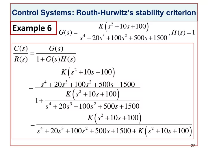
2 K s 10 s 100 4 3 2 s 20 s 100 s 500 s - - PowerPoint PPT Presentation

25

 

2 4 3 2

10 100 ( ) , ( ) 1 20 100 500 1500 K s s G s H s s s s s        

       

2 4 3 2 2 4 3 2 2 4 3 2 2

( ) ( ) ( ) 1 ( ) ( ) 10 100 20 100 500 1500 10 100 1 20 100 500 1500 10 100 20 100 500 1500 10 100 C s G s R s G s H s K s s s s s s K s s s s s s K s s s s s s K s s                           Control Systems: Routh-Hurwitz’s stability criterion

Example 6

26 4 3 2

( ) 20 (100 ) (500 10 ) 1500 100 B s s s s K s K K        

3 1 3 4 2 3 1

20 500 10 1 100 1500 100 20 500 10 a a K a a a K K a a K       

3

100( 7.8)( 192.2) K K    

The value of ∆1=20 >0 and the value of ∆2=1500+10K >0,

7.8 < K < 192.2 conditions for stability

Control Systems: Routh-Hurwitz’s stability criterion

Example 6 Method I using determinants

27 4 2 1 3 1 2 3 2 4 1 3 3 3 3 3 3 1 3 3 n n n

• n

s a a a s a a a a a a a a s b b a a b a b a s b

   

   

4 3 2

( ) 20 (100 ) (500 10 ) 1500 100 B s s s s K s K K        

Control Systems: Routh-Hurwitz’s stability criterion

Example 6 Method II using array

28

1 2 3

1 100 1500 100 20 500 10 1500 10 1500 100 20 100( 7.8)( 192.2) 1500 10

n n n n

s K K s K K s K K K s K

  

       

7.8 < K < 192.2 conditions for stability

Control Systems: Routh-Hurwitz’s stability criterion

Example 6 Method II using array

29

4 3 2

( ) , ( ) 1 K G s H s s s s s     

4 3 2 4 3 2 4 3 2

( ) ( ) ( ) 1 ( ) ( ) 1 C s G s R s G s H s K s s s s K s s s s K s s s s K               

4 3 2

( ) B s s s s s K     

Control Systems: Routh-Hurwitz’s stability criterion

Example 7

30

3

1 1 1 1 1 1 K  

∆1=1 >0 and the value of ∆2=0. ∆3=-K The system is unstable for all values of K

Control Systems: Routh-Hurwitz’s stability criterion

Example 7

Method I using determinants

31

Control Systems: Routh-Hurwitz’s stability criterion

Example 7

Method II using array

4 2 1 3 1 2 3 2 4 1 3 3 3 3 3 3 1 3 3 n n n

• n

s a a a s a a a a a a a a s b b a a b a b a s b

   

  

4 3 2

( ) B s s s s s K     

32

4 3 2 1

1 1 1 1 1 s K s s K K s s K   

The system is unstable for all values

• f K

Control Systems: Routh-Hurwitz’s stability criterion

Example 7

Method II using array

1

ME 779 Control Systems

Controller Basics

Topic #14

Reference textbook:

Control Systems, Dhanesh N. Manik, Cengage Publishing, 2012

2

Learning Objectives

• Proportional controllers
• Proportional and derivative controllers
• Proportional and integral controllers
• Proportional, integral and derivative controllers

Control Systems: Controller Basics

Block diagram

3

Closed-loop (feedback) systems

Control Systems: Controller Basics

4

Proportional controller for inertia load

Proportional control system for inertia load

Proportional controller

Control Systems: Controller Basics

5

2 2 2 2 2

( ) ( ) ( ) 1

p p p p p n

K K K C s Js K R s Js K J s Js        Closed-loop response

p n

K J  

( ) 1 cos

n

c t t   

Step response

Control Systems: Controller Basics

Proportional controller for inertia load

6

Step response

Control Systems: Controller Basics

Proportional controller for inertia load

7

Proportional plus derivative controller for inertia load

Proportional plus derivative controller Proportional and derivative control for inertial load

Control Systems: Controller Basics

d d p

K T K 

8

( ) (1 )

c p d

G s K T s  

2 2 2 2

(1 ) (1 ) ( ) (1 ) ( ) (1 ) 1 (1 )

p d p d p d p d p d p d p

K T s K T s C s Js K T s R s Js K T s Js K T s K T K J s s J J                  

 

2 2 2 2

( ) 1 cos sin 1 1 sin 1 1

n n

p t d d n p d t n n

K c t e t t J K T e t J

 

        

 

                                  

Step response

Control Systems: Controller Basics

Proportional plus derivative controller for inertia load

p n

K J  

2

p d

K T J  

9 2 2 2

(1 ) ( ) (1 ) ( ) 1 (1 ) ( )

p d p d p d p d p

K T s C s Js cs K T s R s Js cs K T s Js s c K T K           

2 2

(1 ) ( ) ( ) ( 2 )

p d n n

K T s C s R s J s s      

Control Systems: Controller Basics

Proportional plus derivative controller for inertia load

1 2

p d p

c K T JK             

10

 

2 2 2 2

( ) 1 cos sin 1 1 sin 1 1

n n

p t d d n p d t n n

K c t e t t J K T e t J

 

        

 

                                  

2

( ) 1

p n

K c J   

Step response

Control Systems: Controller Basics

Proportional plus derivative controller for inertia load Derivative control adds damping to the system

11

1

1

p

K G s  

2

( 1)

i

K G s s  

2 2 2

( ) 1 1 ( 1) ( ) 1 ( ) 1 1 ( 1)

i

E s s s K R s G s s s s s         

1 1

( ) 1 1 ( ) 1 ( ) 2 E s s R s G s s     

Control Systems: Controller Basics

Comparison of proportional and integral controllers

Proportional Integral

12

1

( 1) ( ) ( ) ( 2)

p

K s U s R s s   

2 2

( 1) ( ) ( ) 1

i

K s U s R s s s    

1( )

1 1 ( ) 1 2

p

C s R s s K s     

2 2 2

( ) 1 1 ( ) 1

i

C s R s s s K s s      

Control Systems: Controller Basics

Comparison of proportional and integral controllers

1 1

( ) 1 1 ( ) 1 ( ) 2 E s s R s G s s     

2 2 2

( ) 1 1 ( 1) ( ) 1 ( ) 1 1 ( 1)

i

E s s s K R s G s s s s s          Proportional Integral

13

Control Systems: Controller Basics

Comparison of proportional and integral controllers

 

1

1 2 ( ) 1 2 t e t e  

0.5 2

3 1 3 ( ) cos sin 2 2 3

t

e t e t t



         

 

1

1 2 ( ) 1 2 t c t e  

0.5 2

1 3 3 ( ) 1 sin cos 2 2 3

t

c t e t t



            

Step response

 

1

1 2 ( ) 1 2 t u t e  

0.5 2

1 3 3 ( ) 1 sin cos 2 2 3

t

u t e t t



            

Proportional Integral

14

Steady-state error for step input

Control Systems: Controller Basics

Comparison of proportional and integral controllers

15

Control Systems: Controller Basics

Comparison of proportional and integral controllers

Plant input for step input

16

Control Systems: Controller Basics

Comparison of proportional and integral controllers

Closed-loop response for step input

17

PI (proportional-integral) controllers

Control Systems: Controller Basics

18

1 1 ( 1)

p i i p

sK K K G K s s s s                 

2 1

( ) 1 ( 1) ( ) 1 ( ) (1 )

p i

E s s s R s G s s s K K       

2

( 1)( ) ( ) 1 ( ) (1 )

p i p i

s sK K U s R s s s K K       

Control Systems: Controller Basics

PI (proportional-integral) controllers

19

2

( ) ( ) 1 ( ) (1 ) ( 1)

p i p i

sK K C s R s s s K K s       

( )

t

e t e 

( ) 1 u t 

 

( ) 1 t c t e  

Step response

Control Systems: Controller Basics

PI (proportional-integral) controllers

20

Control Systems: Controller Basics

PI (proportional-integral) controllers

Steady-state error for step input

21

Control Systems: Controller Basics

PI (proportional-integral) controllers

Plant input for step input

22

Control Systems: Controller Basics

PI (proportional-integral) controllers

Closed-loop response for step input

Integral control reduces steady- state error

23

PID (proportional integral derivative) controllers

1

i p d

T K T s s        

d d p

K T K 

i i p

K T K 

Control Systems: Controller Basics

24

Control Systems: Controller Basics

PID (proportional integral derivative) controllers

Consider a unity feedback system given by the following transfer function:

2

80 ( ) 8 80

p

G s s s   

. Design a PID controller such that the steady-state error for step excitation is zero and 10% for ramp excitation, rise time of 0.05 s and maximum

• vershoot of less than 3%.

Example

25

Control Systems: Controller Basics

PID (proportional integral derivative) controllers

Example

2

80 ( ) 8 80

p

G s s s   

Plant transfer function ( ) 1

i c p d

T G s K T s s          Controller transfer function

26

Control Systems: Controller Basics

PID (proportional integral derivative) controllers

Example

 

2 2

80 ( ) ( ) ( ) ( 8 80)

p d i c p

K s T s T G s G s G s s s s      

Forward transfer Function Type 1 system

   

2 3 2

80 ( ) ( ) 8 (1 10 ) 80 (1 ) 80

P d i P d P P i

K T s s T C s R s s s K T s K K T        

Closed-loop response function

27

Control Systems: Controller Basics

PID (proportional integral derivative) controllers

Example

1 1 0.1

e v P i

S K K T   

steady-state error due to ramp excitation

10

P i

K T 

2 2 2 2 2 2

ln( ) ln(0.03) 0.7448 ln( ) ln(0.03)

p p

M M        

 

2 2

80 ( ) ( 8 80)

lim lim

p d i v P i s s

K s T s T K sG s K T s s

 

      

Velocity error

28

Control Systems: Controller Basics

PID (proportional integral derivative) controllers

Example

2 2 1 1

1 1 0.7448 tan tan 0.7306 (41.86 ) 0.7448 rad   

 

    

0.7306 48.2207 / 0.05

d r

rad s t         

2 2

48.2207 72.2642 / 1 1 0.7448

d n

rad s        

29

Control Systems: Controller Basics

PID (proportional integral derivative) controllers

Example

Since the characteristic equation of closed- response is cubic in nature, at least one of the roots will be real and the other roots may be real

• r complex. But since we prefer to have at least
• ne set of complex roots that will give the desired
• scillatory and exponentially decaying response,

we can assume that one root is real and the other two roots are complex.

30

Control Systems: Controller Basics

PID (proportional integral derivative) controllers

Example

 

 



3 2 2 2

8 (1 10 ) 80 (1 ) 80 2

P d P P i n n

s s K T s K K T s a s s           

 

 



3 2 2

8 (1 10 ) 80 (1 ) 80 107.6453 5222.1

P d P P i

s s K T s K K T s a s s         

31

Control Systems: Controller Basics

PID (proportional integral derivative) controllers

Example

   

8 1 10 107.6453 80 1 107.6453 5222.1 80 5222.1

P d P P i

K T a K a K T a       

64.4824 0.0193 0.1551 0.1532

P d i

K T T a    

10

P i

K T 

Control Systems: Controller Basics

Conclusion

1

ME 779 Control Systems

Hydraulic Controllers

Topic #15

Reference textbook:

Control Systems, Dhanesh N. Manik, Cengage Publishing, 2012

2

Control Systems: Hydraulic Controllers

Learning Objectives

• Dashpot
• derivative action
• integral action
• Proportional and integral controllers
• Proportional and derivative controllers
• Dashpots connected in series
• Proportional, integral and derivative controllers

3

DASHPOT

1 2

P P q R  

q: flow rate P1, P2 pressures R: resistance

Control Systems: Hydraulic Controllers

4

DASHPOT: derivative action

1 2

( ) F A P P  

1 2

( ) A P P kz  

dy dz q dt dt A  

( ) qdt A dy dz   

Control Systems: Hydraulic Controllers

5

DASHPOT: derivative action

2

dy dz kz dt dt RA   

2

( ) ( ) Z s s k Y s s RA   

2

RA k   

( ) ( ) 1 Z s sY s s    

The output has to be integrated to be compared with the input and hence the derivative action

• f the dashpot (you can only

compare apples with apples at the summing point)

Control Systems: Hydraulic Controllers

s 

6

DASHPOT- integral action

1 2

( ) ( ) k y z A P P   

qdt A dz  

1 2

P P q R  

Control Systems: Hydraulic Controllers

7

DASHPOT- integral action

( ) 1 ( ) 1 Z s Y s s   

2

RA k   

The output has to be differentiated to be compared with the input and hence the integral action of the dashpot (you can only compare apples with apples at the summing point)

Control Systems: Hydraulic Controllers

s 

8

Hydraulic proportional plus integral controller

Control Systems: Hydraulic Controllers

Derivative action in the feedback loop

9

Hydraulic proportional plus integral controller

Control Systems: Hydraulic Controllers

1 s s   

10

( ) ( ) ( ) ( ) 1 1 ( ) ( 1) ( )( 1) b K b K Y s a b s a b s Ka s Ka X s a b s s a b s              

Control Systems: Hydraulic Controllers

Hydraulic proportional plus integral controller

11

( ) ( 1) 1 1 ( ) Y s b s b X s a s a s             

Control Systems: Hydraulic Controllers

Hydraulic proportional plus integral controller

12

Hydraulic proportional plus derivative controller

Control Systems: Hydraulic Controllers

Integral action in the feedback loop

13

Control Systems: Hydraulic Controllers

Hydraulic proportional plus derivative controller

1 1 s  

14

( ) ( ) ( ) 1 ( ) ( 1) b K Y s a b s Ka X s a b s s      

 

( ) 1 ( ) Y s b s X s a   

Control Systems: Hydraulic Controllers

Hydraulic proportional plus derivative controller

15

Hydraulic proportional-integral- derivative controller

Control Systems: Hydraulic Controllers

Derivative Integral

16

Dashpots connected in series

Control Systems: Hydraulic Controllers

Hydraulic proportional-integral- derivative controller

Derivative Integral

17

1 1 2

( ) k z A P P  

1 2 1 1

P P q R  

1 1 1

k z AR q 

2 1 2 3 4

( ) ( ) ( ) k y u A P P A P P     

1

( ) q dt A du dz   

1

du dz q A dt dt         

Control Systems: Hydraulic Controllers

Hydraulic proportional-integral- derivative controller

Dashpots connected in series

18

3 4 2 2

P P q R  

1

q du dz dt A dt   

1 2 1

k z du dz dt R A dt   

1

du z dz dt dt   

2

q dt A du  

2

du q A dt  

2 1 1 1

R A k   

Control Systems: Hydraulic Controllers

Hydraulic proportional-integral- derivative controller

Dashpots connected in series

19

3 4 3 4 2 2 2 2

( ) P P A P P q du dt A R A R A        

3 4 2 2

( ) A P P du dt k   

2 1 2 2

( ) du k y u k z k dt    

2 2 2 2

R A k   

Control Systems: Hydraulic Controllers

Hydraulic proportional-integral- derivative controller

Dashpots connected in series

20

2 2 1 2 2

du k y k u k z k dt    

 

2 2 2 2 1

( ) ( ) ( ) k Y s U s k k s k Z s    

1

( ) 1 ( ) Z s U s s s         

1 1

1 ( ) ( ) s U s Z s s          

Control Systems: Hydraulic Controllers

Hydraulic proportional-integral- derivative controller

Dashpots connected in series

21

 

1 2 2 2 1 1

1 ( ) 1 ( ) s k Y s k s k Z s s                   

1 2 1 1 2 1 2 1 2

( ) ( ) ( ) 1 s Z s Y s k s s s k                 

Control Systems: Hydraulic Controllers

Hydraulic proportional-integral- derivative controller

Dashpots connected in series

22

1 2 2 1

k k   

1 2 1 2 1 2

( ) ( ) ( 2 ) 1 s Z s Y s s s             

Control Systems: Hydraulic Controllers

Hydraulic proportional-integral- derivative controller

Dashpots connected in series

23

Control Systems: Hydraulic Controllers

Hydraulic proportional-integral- derivative controller

24 1 2 1 2 1 2

( ) ( ) ( ) 1 ( ) ( 2 ) 1 b K Y s a b s s Ka X s a b s s s                

1 2 1 2 1 2

1 ( ) ( 2 ) 1 s Ka a b s s s              

Control Systems: Hydraulic Controllers

Hydraulic proportional-integral- derivative controller

D.N. Manik 25

2 2 1 1

2 ( ) 1 1 ( ) Y s b s X s a s                    

2 1 1 2

2 1 1

p I D

b K a b K a b K a              

( ) ( )

I p D

K Y s K K s X s s   

Control Systems: Hydraulic Controllers

Hydraulic proportional-integral- derivative controller