7. Artificial neural networks Introduction to neural networks - - PDF document

101 | P a g e

• 7. Artificial neural networks

Introduction to neural networks

Despite struggling to understand intricacies of protein, cell, and network function within the brain, neuroscientists would agree on the following simplistic description of how the brain computes: Basic units called "neurons" work in parallel, each performing some computation on its inputs and passing the result to other neurons. This sounds trivial, but borrowing and simulating these essential features

• f the brain leads to a powerful computational tool called an artificial neural network. In studying

(artificial) neural networks, we are interested in the abstract computational abilities of a system composed of simple parallel units. Although motivated by the multitude of problems that are easy for animals but hard for computers (like image recognition), neural networks do not generally aim to model the brain realistically. In an artificial neural network (or simply neural network), we talk about units rather than neurons. These units are represented as nodes on a graph, as in Figure []. A unit receives inputs from other units via connections to other units or input values, which are analogous to synapses. The inputs might represent, for instance, pixels in an image that the network must classify as a dog or a cat. If we focus on one particular unit, the connections that point to it are like dendrites—they bring information to the unit from others. Some connections have more influence

• n the unit, and some may actually act in opposing

directions—just like there are excitatory and inhibitory synapses of varying strengths and at varying locations on a

• neuron. In biology, this would be referred to as synaptic

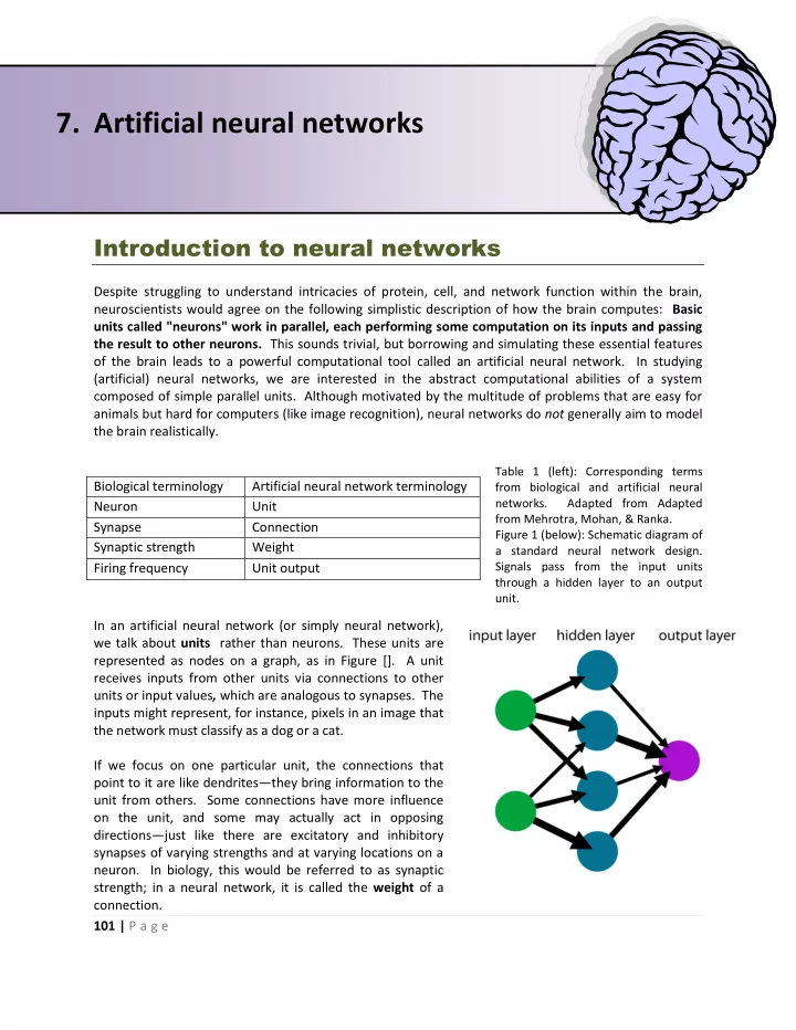
strength; in a neural network, it is called the weight of a connection. Biological terminology Artificial neural network terminology Neuron Unit Synapse Connection Synaptic strength Weight Firing frequency Unit output

Table 1 (left): Corresponding terms from biological and artificial neural

• networks. Adapted from Adapted

from Mehrotra, Mohan, & Ranka. Figure 1 (below): Schematic diagram of a standard neural network design. Signals pass from the input units through a hidden layer to an output unit.

102 | P a g e The connections pointing away from a unit are like its axon—they project the result of its computation to other units. This output is analogous to the firing rate of a neuron. The neural networks we will study work on an arbitrary timescale and do not “fire action potentials,” although some types of neural networks do. There are many types of neural networks, specialized for various applications. Some have only a single layer of units connected to input values; others include “hidden” layers of units between the input and final output, as shown in Figure 1. If there are multiple layers, they may connect only from one layer to the next (called a feed-forward network), or there may be feedback connections from higher levels back to lower ones, as we see in cortex. Neural networks can “learn” in several ways:  Supervised learning is when example input-output pairs are given and the network tries to agree with these examples (for instance, classifying coins based on weight and diameter, given labeled measurements of pennies, nickels, dimes, and quarters)  Reinforcement learning is when no “correct” answer is given along with the input data, but the network’s performance is “graded” (for instance, it might win or lose a game of chess)  Unsupervised learning is when only input data are given to the network, and it finds patterns without receiving direct feedback (for instance, recognizing that there are four types of coins without assigning the labels “penny,” “nickel,” “dime,” “quarter”) We will focus on supervised learning. They can also perform “association” tasks, for instance reproducing a full image from a small piece.

The learning problem

If you show a picture to a three-year-old and ask him if there is a tree in it, he is likely to give you the right answer. If you ask a thirty-year-old what the definition of a tree is, he is likely to give you an inconclusive answer. We didn't learn what a tree is by studying the mathematical definition of trees. We learned it by looking at a lot of trees. In other words, we learned from data. Yaser Abu-Mostafa Neural networks are most commonly used to “learn” an unknown function. For instance, say you want to classify email messages as spam or real. The ideal function is one that always agrees with you, but you can’t describe exactly what criteria you use. Instead, you use that ideal function—your own judgment—on a randomly selected set of messages from the past few months to generate training

• examples. Each training example is simply an email message with a correct label, either “spam” or

“real.” You decide to automatically classify the message based on how many times each word on a list appears. You will multiply each frequency by some value, add up these products, and if they exceed some threshold, the message will be labeled spam. Your strategy provides you with a set of candidate rules (corresponding to the possible multipliers and thresholds) for deciding whether a message is spam. Learning then consists of using the training examples to pick the best rule from this set. (There might be

103 | P a g e better ideas, for instance taking into account grammar or the sender’s email address, but we aren’t concerned with those during the formal process of learning.) Once you come up with a rule, its performance is evaluated on a test set. The test set is essentially a spare training set: it consists of inputs (in this case emails) with correct labels (“spam” or “real”). You use your rule to classify the inputs in the test set and compare the results to the correct labels to see how you did. This is a crucial step that allows us to estimate how well our rule will do when we start using it on our email. Because we have specifically worked to make our rule agree with the training examples, its performance on those training examples is artificially inflated. Your rule may perform slightly better or worse on the test set than on emails in general, but at least this estimate of its performance is unbiased. In order to draw meaningful conclusions from the test set, we need to be careful not to contaminate it by using it to select a rule. If our rule doesn’t do well on the test set and we go back to adjust it, we need to use a new test set. You can think of training examples as last year’s exam that you study from, and the test set as the actual exam your teacher gives. Making sure you can do all of last year’s problems should improve your grade, but being able to do all of the practice problems (after seeing the answers!) doesn’t mean you’ve mastered the subject. And if you do poorly on the exam and your teacher lets you retake it, you shouldn’t get the same questions again! It may seem strange that we can learn a completely unknown function with any confidence. The key is that the training and testing examples are selected randomly from the same population of inputs we care about being able to process correctly. Using laws of probability, we can put an upper bound on the chance that the “out-of-sample” (non-training) error will be very different from the “in-sample” (training) error.

Linear threshold units

The rule we described for classifying emails was actually a computation that could be performed by a “artificial neuron” called a linear threshold unit (LTU), shown in Figure 2.

LTU

x0 = -1 x2 x3 x1 xn … w0 w2 w1 … w3 wn s f(s)

104 | P a g e An LTU receives scalar inputs

1 2

, , , ,

n

x x x x and first computes the weighted sum

1 1 2 2 n n

s w x w x w x w x     

. (We could also write this as

i n i i i

w x

 



• r the dot product

 w x .) If

s 

, then the LTU outputs f(s) = 1; otherwise, it outputs f(s) = -1. This is known as a “hard threshold” and represents a decision about or classification of the input data. Many neural networks use a soft thresholding function, in which the output is always between -1 and 1 but does not “jump” from

• ne to the other.

The input

x is special; it is always 1  . This effectively implements a nonzero threshold for the

weighted sum of the actual inputs. At the boundary between the neuron outputting -1 and 1,

s 

, so

1 1 2 2 1 1 2 2 1 1 2 2 n n n n n n

w x w x w x w x w w x w x w x w x w x w x w               

The special weight

w is often called the LTU’s threshold. The plane of values

1 2 3

( , , , , )

n

x x x x

that leads to

s 

is called the decision boundary because on one side the LTU outputs 1 and on the other side it outputs -1. An important consequence of using the weighted sum s is that an LTU can only learn to distinguish between sets that are indeed separated by some plane, as shown in Figure 3. Let’s do an example computation of an LTU’s output. Here is a unit that receives two inputs besides

x :

In this case,

3 ( 1) 1 5 ( 1) 0 2 s         

, which is positive, so

( ) 1 f s  . The decision boundary is

shown in Figure 4.

LTU

• 1

5 3

• 1

1 s f(s) x2

Figure 3: A single LTU could distinguish between circles and triangles only in the case on the left. In the

• ther two examples, there

is no line dividing the two groups.

105 | P a g e In class, we will study the perceptron learning rule, which provides a way to adjust the weights of an LTU based on a training set. As long as it is possible for an LTU to distinguish between the input classes, the perceptron learning rule will eventually find a correct decision boundary.

Storing memories in a neural network

Besides learning unknown functions, neural networks can also be used to associate an input pattern (for instance, an incomplete or corrupted version of an image) with a stored “memory.” This is a common problem in everyday life: we associate people’s names with their faces and other characteristics, for instance, and can often call up a complete song (“by the dawn’s early light”) or story (“and he puffed and he blew the house down!”) from just a few notes or words. Children practice their animal sounds (“What does the dinosaur say?”) before they even have experience with the animals. We will study one of the most commonly used implementations of “memory” in an artificial neural network, a discrete Hopfield network. This network is made up of connected linear threshold units (the

• utput of one becomes the input to another) whose output can be either -1 or 1 at any given time. A

memory then corresponds to a state of the network, meaning the current output of each unit. One natural type of memory for a discrete Hopfield network is a binary image, in which each pixel (a unit) is either white (output 1) or black (output -1).

                

x1

( ) 1 f s   ( ) 1 f s  Figure 5: Decision boundary for the LTU shown in Figure 4. To find the boundary we set s  , so

1 2 1 2

3 ( 1) 1 ( 1) 3 x x x x          

Check a few points, such as (5,0) as shown in the example in Figure 4, to check that the decisions shown

• n this plot agree with the output of the LTU.
• 1

1

• 1
• 1
• 1

1 Figure 6: A small discrete Hopfield network (left) and the image its state represents (right). The current output

• f each unit is represented by its

color, black (-1) or white (1). For clarity, connections between the units are either -1 (black arrows) or 1 (white arrows).

106 | P a g e Units are updated one at a time in random order until the state of the network stops changing. The input to a Hopfield network is the initial pattern, and the output is this stable (unchanging) state. As an example, consider updating the bottom right node in Figure 6: The weighted sum of the inputs is

1( 1) 1(1) 1( 1) 1(1) 1( 1) 5         

, which is positive, so the output should change to 1. Should any

• f the other outputs change?

In class we will learn how to choose the weights to ensure that one or more images are stable states of the network. Then when an input (initial image) is presented, the network will proceed to the most similar stored image. We will only consider Hopfield networks with symmetric weights, meaning that the weight from unit A to unit B is the same as the weight from unit B to unit A.

Chapter resources Vocabulary

Unit Weight Supervised learning Reinforcement learning Unsupervised learning Training examples Test set Learning Linear threshold unit (LTU) Decision boundary Threshold Hopfield network Stable state

• +
• +

107 | P a g e

LAB 7: Human linear threshold units

Training a Perceptron

You will be working in pairs to train linear threshold units to recognize colors using the Perceptron learning rule (taught in class).

• 1. Choose one partner to start as the LTU, and one to start as the trainer (you’ll switch). Obtain a

rule card for the trainer. The trainer will know the actual rule the LTU should implement and will say whether the LTU’s output is correct or incorrect after each training example.

• 2. The trainer should split the pile of example cards into a training set (~2/3) and a test set (~1/3).

Set the test set aside.

• 3. Go through the entire training deck twice, shuffling the cards in between. For each card,
• a. The trainer looks at the color and makes a decision based on his/her rule regarding what

the output of the LTU should be (1 or -1). For instance, if the rule card says “This color looks either red or green” and the color looks purple, the output should be -1. The trainer does NOT show the color to the LTU.

• b. The trainer reads the input values to the LTU. The first input value is always -1 to

implement a possibly nonzero threshold, as discussed in the reading. The remaining three inputs are red, green, and blue light intensities.

• c. The LTU computes the weighted sum s based on the current weights (initially all zero).

If s is nonnegative, the output is 1; otherwise the output is -1.

• d. The trainer tells the LTU whether the output was correct or not. If the output was

incorrect, the LTU needs to increment the weights by 0.1 y

 x, where y is the correct

• utput and the vector x is the input pattern. In this case the learning rate is 0.1.

The LTU should keep track of the computations for each input in the tables provided.

• 4. Put aside the training deck and move to the test deck. Now the weights of the LTU are set and

will no longer vary—we just want to see how well it agrees with the rule on examples it’s never seen before.

• 5. Finally, the trainer can tell the LTU what the “true” or “target” rule was. Then switch roles with

a fresh rule card.

108 | P a g e TRAINING Input Weights s Output Correct? Change weights by… (-1, (0, 0, 0, 0)

109 | P a g e TESTING Final weights: Input s Output Correct?

110 | P a g e

Human Hopfield network

In this part we will go outside to simulate the function of a Hopfield network with two stored images. The weights for the network have already been computed, and you will be exploring the behavior of the network to discover the stable states. Each student will act as one unit or “pixel” in an image. You have a piece of posterboard which can be placed white-side-up to signal output 1 or black-side-up to signal output -1. Along with your posterboard will be instructions on how to update your pixel. 1) Start with the initial pattern that has been set up and find one stable state by allowing the “neurons” to repeatedly update their values until no one needs to change his/her output value

• anymore. Record the input and output patterns.

2) Repeat the process of finding a stable state from a different initial pattern the instructors will set

• up. Record the input and output patterns.

3) Explore which input patterns map to which outputs:

• a. Start from one of the stable states and have only one student flip his/her posterboard,

then proceed to update until you reach a stable state.

• b. Start from one of the stable states and have four students flip their posterboards. Do

you still reach the same state? What if you choose another four students?

• c. Start from one of the stable states and have ALL of the students flip their posterboards.

111 | P a g e

Human LTU homework

Part A: Perceptrons 1) What was the first rule your LTU tried to learn? a) Summarize its performance on the training set by plotting the fraction of correct decisions against the training example number (group five examples together). b) How well did it do on the test set (percentage correct)? c) Did it “learn” the secret rule? How might you have improved its performance? 2) What was the second rule your LTU tried to learn? a) Summarize its performance on the training set by plotting the fraction of correct decisions against the training example number (group five examples together). It turns out this one was impossible for a single LTU to compute. Do you have evidence that it wasn’t able to learn this rule? b) Draw a neural network made up of multiple LTUs that could learn this second rule. You may describe what each unit computes in words rather than giving exact weights. Part B: Hopfield network 3) Prove that if a state of a Hopfield network is stable, so is its “inverse” (with the output of each unit flipped from 1 to -1 or vice versa). 4) How accurate would you guess your classmates were in their arithmetic? Why could we reach a stable state without requiring that none of 24 students would make a mistake during the updates?