
SLIDE 1
CVG-UPM
COMPUTER VISION
Machine Learning and Neural Networks
- P. Campoy
- P. Campoy
Machine Learning & Neural Networks
7.- Non supervised Neural Networks: Self-organizing Maps
by Pascual Campoy Grupo de Visión por Computador U.P.M. - DISAM
3
CVG-UPM
COMPUTER VISION
Machine Learning and Neural Networks
- P. Campoy
- P. Campoy
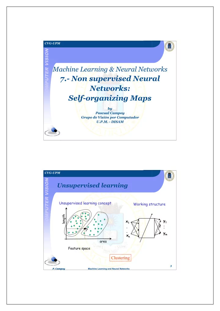
Unsupervised learning
Feature space
Unsupervised learning concept
?
area length