A C A Core R Robot Al Algorithm hm: I Inverse K Kinematics - - PowerPoint PPT Presentation

a c a core r robot al algorithm hm i inverse k
SMART_READER_LITE
LIVE PREVIEW

A C A Core R Robot Al Algorithm hm: I Inverse K Kinematics - - PowerPoint PPT Presentation

A C A Core R Robot Al Algorithm hm: I Inverse K Kinematics Setting a robots joints so end effector reaches a target Input: current robot geometry Output: required joint increments Computationally intensive problem all limbed


slide-1
SLIDE 1

1

A C A Core R Robot Al Algorithm hm: I Inverse K Kinematics

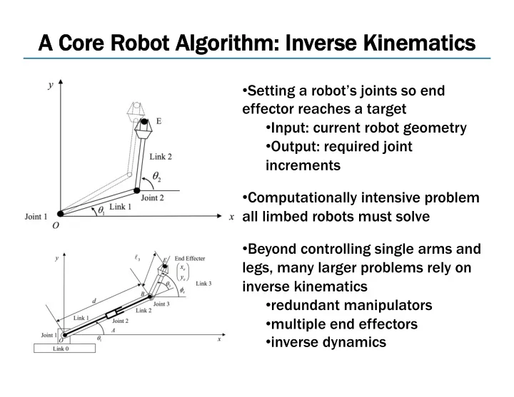
  • Setting a robot’s joints so end

effector reaches a target

  • Input: current robot geometry
  • Output: required joint

increments

  • Computationally intensive problem

all limbed robots must solve

  • Beyond controlling single arms and

legs, many larger problems rely on inverse kinematics

  • redundant manipulators
  • multiple end effectors
  • inverse dynamics
slide-2
SLIDE 2

2

A D A Digital A Accelerator f for I Inverse K Kinematics

  • Inverse kinematics not well suited for normal digital

architectures – Entirely floating point array, matrix operations – 40% of cycles in inverting matrices – 15% of cycles in sine, cosine operations

  • We solve IK via damped least squares

– Dedicated sine, cosine function generators – Parallel, fixed-point functional units – Solves IK problem in 100µs: compare against 10ms for general algorithm on CPU

slide-3
SLIDE 3

3

Ar Archi hitecture a and Toolcha hain

FPGA CONFIGURATION TIME FPGA RUNTIME LINUX RUNTIME

Target Pose Incremental Joint Actions ROS URDF Collada D-H Params Robot Geometry XML matrix constants variables Forward Kinematics Jacobian Jacobian Block Forward Kinematics Matrix Damped Least Squares Block Inverse Kinematics Matrix cpp-inverse- kinematics- library Compiler Robot Current Joint Pose Full Matrix

  • Mult. Pipeline
4x4 Matrix Multiplier d A α Θ 16 16
  • axis of rot. / trans.
  • pos. & rot. of joint
16 A*cos(Θ) A*sin(Θ) sin(Θ)sin(α)
  • sin(Θ)cos(α)
  • cos(Θ)sin(α)
cos(Θ)cos(α) sin(Θ) cos(Θ) sin(α) cos(α) Θ α A d Jacobian Finder 16

...

slide-4
SLIDE 4

4

Ar Archi hitecture a and T Timing D Design

  • Architectural Choices
  • Pipelining sine/cosine and array multiply
  • Parallelized matrix multiply and matrix inversion
  • Fixed point representations throughout system
  • Timing Choices
  • Single array of multipliers shared amongst modules
  • Aggregate individual enable and done signals into

global state machine

slide-5
SLIDE 5

5

Experiences a and I Issues

  • Deciding on the algorithm to use
  • Determining what implementation would fit on

the board

  • Convincing ourselves the algorithm works
  • Extensively tested the core hardware, but not the

top-level interface (until yesterday)

slide-6
SLIDE 6

6

Lessons L Learned

  • Test the whole stack earlier
  • Plan before trying to implement
  • Use timing diagrams and area estimates before

touching hardware

  • Leave no ambiguity in the design