A Crash Course on Programmable Graphics Hardware Li-Yi Wei - - PDF document

A Crash Course on Programmable Graphics Hardware

Li-Yi Wei Microsoft Research Asia

Abstract

Recent years have witnessed tremendous growth for programmable graphics hardware (GPU), both in terms of performance and func-

• tionality. In this paper, we overview the high-level architecture of

modern GPU, and introduce the GPU programming model. We also briefly describe the kinds the visual effects and applications that can be achieved by programmable graphics hardware. Keywords: Programmable Graphics Hardware

1 Introduction

Programmable graphics hardware is one of the few technologies that have survived through the ashes of the 90s dot com bubble burst, and it is still advancing at warp speed today. Just a few years ago, when SGI still dominated, graphics hardware is almost syn-

• nymous to super computer and people were charmed by these huge

machine boxes (you get a sense of this feeling by the name Onyx

• f one of SGIs last workstations). However, as new generations
• f semiconductor process waved by, the entire graphics pipe has

been shrunken from an entire machine to a single chip. Nowadays, graphics hardware is no longer a luxury item. In contrast, everyone and their brothers seem to have the latest graphics cards to play the hottest games, and it almost seems a shame if you dont have one as

• well. But you probably dont have to worry about this anyway, since

it is almost impossible to buy a computer today without the latest graphics chips from either ATI or NVIDIA. In this paper, we introduce programmable graphics hardware. Our goal is to enable you have fun with graphics chips, so we

• nly describe high level architecture that are just enough for you

to know how to program. In particular, we concentrate on the two programmable stages of the graphics pipeline: the vertex and frag- ment processor, describe their programming model, and demon- strate possible applications with these programmable units.

2 Graphics Hierarchy

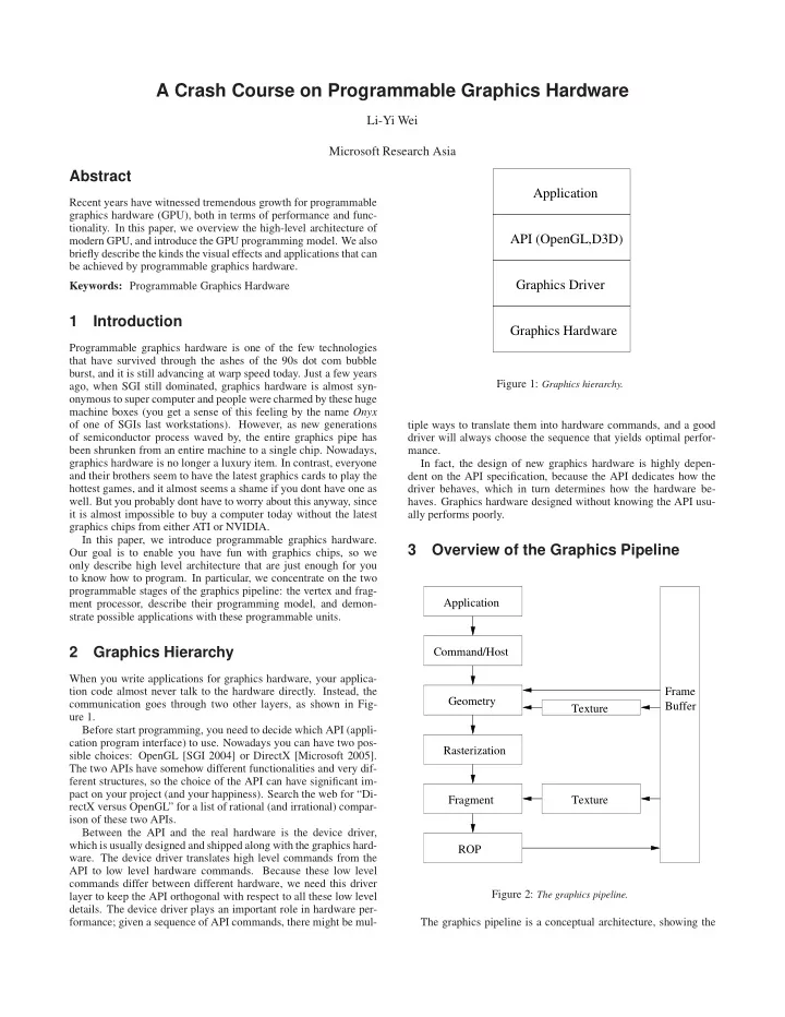
When you write applications for graphics hardware, your applica- tion code almost never talk to the hardware directly. Instead, the communication goes through two other layers, as shown in Fig- ure 1. Before start programming, you need to decide which API (appli- cation program interface) to use. Nowadays you can have two pos- sible choices: OpenGL [SGI 2004] or DirectX [Microsoft 2005]. The two APIs have somehow different functionalities and very dif- ferent structures, so the choice of the API can have significant im- pact on your project (and your happiness). Search the web for “Di- rectX versus OpenGL” for a list of rational (and irrational) compar- ison of these two APIs. Between the API and the real hardware is the device driver, which is usually designed and shipped along with the graphics hard-

• ware. The device driver translates high level commands from the

API to low level hardware commands. Because these low level commands differ between different hardware, we need this driver layer to keep the API orthogonal with respect to all these low level

• details. The device driver plays an important role in hardware per-

formance; given a sequence of API commands, there might be mul-

Graphics Driver Graphics Hardware API (OpenGL,D3D) Application

Figure 1: Graphics hierarchy. tiple ways to translate them into hardware commands, and a good driver will always choose the sequence that yields optimal perfor- mance. In fact, the design of new graphics hardware is highly depen- dent on the API specification, because the API dedicates how the driver behaves, which in turn determines how the hardware be-

• haves. Graphics hardware designed without knowing the API usu-

ally performs poorly.

3 Overview of the Graphics Pipeline

Texture Application Command/Host Geometry Rasterization Fragment Texture ROP Buffer Frame Figure 2: The graphics pipeline. The graphics pipeline is a conceptual architecture, showing the

basic data flow from a high level programming point of view. It may or may not coincide with the real hardware design, though the two are usually quite similar. The diagram of a typical graphics pipeline is shown in Figure 2. The pipeline is consisted of multiple functional stages. Again, each functional stage is conceptual, and may map to one or multiple hardware pipeline stages. The arrows indicate the directions of major data flow. We now describe each functional stage in more detail.

3.1 Application

The application usually resides on a CPU rather than GPU. The application handles high level stuff, such as artificial intelligence, physics, animation, numerical computation, and user interaction. The application performs necessary computations for all these ac- tivities, and sends necessary command plus data to GPU for render- ing.

3.2 Host

The host is the gate keeper for a GPU. Its main functionality is to receive commands from the outside world, and translates them into internal commands for the rest of the pipeline. The host also deals with error condition (e.g. a new glBegin is issued without first issuing glEnd) and state management (including context switch). These are all very important functionalities, but most programmers probably dont worry about these (unless some performance issues pop up).

3.3 Geometry

The main purpose of the geometry stage is to transform and light

• vertices. It also performs clipping, culling, viewport transforma-

tion, and primitive assembly. We now describe these functionalities in detail. 3.3.1 Vertex Processor The vertex processor has two major responsibilities: transformation and lighting. In transformation, the position of a vertex is transformed from the object or world coordinate system into the eye (i.e. camera) coordinate system. Transformation can be concisely expressed as follows:

  

xo yo zo wo

  

= M

  

xi yi zi wi

  

(1) (2) Where ( xi yi zi wi ) is the input coordinate, and ( xo yo zo wo ) is the transformed coordinate. M is the 4 × 4 transformation matrix. Note that both the input and out- put coordinates have 4 components. The first three are the familiar x, y, z Cartesian coordinates. The fourth component, w, is the ho- mogeneous component, and this 4-component coordinate is termed homogeneous coordinate. Homogeneous coordinates are invented mainly for notational convenience. Without them, the equation above will be more complicated. For ordinary vertices, the w com- ponent is simply 1. Let me give you some more concrete statements of how all these means. Assuming the input vertex has a world coordi- nate ( xi yi zi ). Our goal is to compute its location in the camera coordinate system, with the camera/eye center located at ( xe ye ze ) in the world space. After some mathematical derivations which are best shown on a white board, you can see that the 4 × 4 matrix M above is consisted of several components: the upper-left 3 × 3 portion the rotation sub-matrix, the upper right 3× 1 portion the translation vector, and the bottom 1× 4 vector the projection part. In lighting, the color of the vertex is computed from the posi- tion and intensity of the light sources, the eye position, the vertex normal, and the vertex color. The computation also depends on the shading model used. In the simple Lambertian model, the lighting can be computed as follows: (¯ n.¯ l)c (3) Where ¯ n is the vertex normal, ¯ l is the position of the light source relative to the vertex, and c is the vertex color. In old generation graphics machines, these transformation and lighting computations are performed in fixed-function hard-

• ware. However, since NV20, the vertex engine has become pro-

grammable, allowing you customize the transformation and light- ing computation in assembly code [Lindholm et al. 2001]. In fact, the instruction set does not even dictate what kind of semantic oper- ation needs to be done, so you can actually perform arbitrary com- putation in a vertex engine. This allows us to utilize the vertex engine to perform non-traditional operations such as solving nu- merical equations. Later, we will describe the programming model and applications in more detail. 3.3.2 Primitive Assembly Here, vertices are assembled back into triangles (plus lines or points), in preparation for further operation. A triangle cannot be processed until all the vertices have been transformed as lit. As a result, the coherence of the vertex stream has great impact on the efficiency of the geometry stage. Usually, the geometry stage has a cache for a few recently computed vertices, so if the vertices are coming down in a coherent manner, the efficient will be better. A common way to improve vertex coherency is via triangle stripes. 3.3.3 Clipping and Culling After transformation, vertices outside the viewing frustum will be clipped away. In addition, triangles with wrong orientation (e.g. back face) will be culled. 3.3.4 Viewport Transformation The transformed vertices have floating point eye space coordinates in the range [−1, 1]. We need to transform this range into window coordinates for rasterization. In viewport stage, the eye space coor- dinates are scaled and offseted into [0, height−1]×[0, width−1].

3.4 Rasterization

The primary function of the rasterization stage is to convert a tri- angle (or line or point) into a set of covered screen pixels. The rasterization operation can be divided into two major stages. First, it determines which pixels are part of the triangle, as shown in Fig- ure /reffig:rasterization-coverage. Second, rasterization interpolates the vertex attributes, such as color, normal, and texture coordinates, into the covered pixels. Specifically, for an attribute ¯ C, it is interpolated as follows: ¯ Cp =

• i=A,B,C
• wi. ¯

Ci (4)

Figure 3: Rasterizing a triangle. The gray pixels are rasterized as inside

• f the triangle.

Where ¯ Ci are the vertex attributes at vertices A, B, C, and wi are the interpolation weight, and ¯ Cp is the interpolated value at the pixel. The weights need to be chosen to ensure continuity cross adjacent

• triangles. The standard method is barycentric coordinates, which

simply assigns weight to a vertex proportional to the opposing tri- angle, as shown in Figure 4.

C A P B

Figure 4: Barycentric coordinate interpolation. The weight for vertex A,

wA, equals to △BP C

△ABC , where △ indicates triangle area. The weights for

vertex B and C are defined similarly.

3.4.1 Perspective Correct Barycentric Interpolation For correct perspective effect, make sure you divide ¯ Ci by their w components in homogeneous coordinates when performing barycentric interpolation as in Equation 4. Otherwise, the inter- polation will appear incorrect for a perspectively projected triangle. This artifact is particularly noticeable for texture coordinates when the applied texture has high frequency content. For colors, since they are in low frequency, the artifact is often not noticeable.

P1 P1, w1 P, w P2, w2 eye P2 P

incorrect

P1/w1 P1, w1 P, w P2, w2 eye P2/w2 P/w

correct Figure 5: Perspective interpolation. Exercise Do you know how a quad is rasterized? Is it rasterized as two triangles, or as an entire rectangle? Write a simple program to figure out how your graphics chip rasterizes a quad. Can you think of any problems with the specific method the quad is raster- ized? Exercise Write a software rasterizer to visualize the perspective interpolation problem. Usually you cannot see this in real graphics hardware, since the rasterization stage is not programmable. Can you figure out a method to visualize the perspective interpolation problem on graphics hardware, via some programming tricks?

3.5 Fragment

Before we introduce the fragment stage, lets first define what frag- ment is. Basically, a fragment corresponds to a single pixel and includes color, depth, and sometimes texture coordinate values.

1

For an input fragment, all these values are interpolated from ver- tex attributes in the rasterization stage, as described earlier. The role of the fragment stage is to process each input fragment so that a new color or depth value is computed. In old generation graph- ics machines, the fragment stage has fixed function and performed mainly texture mapping. Between NV20 and NV30, the fragment stage has become reconfigurable via register combiners. But this is all old stuff and I dont think you need to worry about it. Since NV30, the fragment stage has become fully programmable just like the vertex processor. In fact, the instruction set of vertex and frag- ment programs are very similar. The major exception is that the vertex processor has more branching capability while the fragment processor has more texturing capability, but this distinction might

• nly be transitory.

Given it is programmability and computation power, fragment processors have been both embraced by the gaming community for advanced rendering effects, as well scientific computing commu- nity for general purpose computation such as numerical simulation [Harris 2005]. Later, we will describe the programming model and applications in more detail.

3.6 Texture

The main purpose of texture stage is to allow texturing to fragments as a cheap way to simulate surface details. Texture unit has two main functionalities. First, it manages a cache for texture data. This is mainly for performance, because reading texture data di- rectly from the frame-buffer can be very slow. Second, texture unit performs filtering of the texture data, such as bilinear, trilinear, and anisotropic filtering. Although in theory all these filtering oper- ations can now be performed inside fragment programs, leaving them in texture has certain performance advantages. In addition, native texture filtering simplifies fragment program as it is a very common operation. As can be seen in Figure 2, texture stage is not drawn as part of the main pipeline. The reason is that texturing is optional and not all applications use it. In applications based on micro-polygons, all the details are encoded in vertex colors and therefore there is no need for texture mapping. Although texture stage is currently not programmable, there ex- ists a wide variety of rendering effects that are achieved through

• texturing. We will describe some of these effects later.

3.7 ROP (Raster Operation)

ROP (Raster Operation) is the unit that writes fragments into the frame-buffer. The main functionality of ROP is to efficiently write batches of fragments into the frame-buffer via compression. It also performs alpha, depth, and stencil tests to determine if the fragments should be written or discarded. ROP deals with sev- eral buffers residing in the frame-buffer, including color, depth, and stencil buffers.

3.8 Frame Buffer

The frame-buffer is the main storage for the graphics pipeline, in addition to a few scattered caches and FIFOs throughout the pipe. The frame-buffer stores vertex arrays, textures, and color, depth,

1In Unreal Tournament, fragment counts the number of opponents you

kill.

stencil buffers. The content of the color buffer is fed to display for viewing. Frame-buffer has several major characteristics: size, width, la- tency, and clock speed. The size determines how much and how big textures and buffers you can store on chip, the width determines how much data maximum you can transfer in one clock cycle, the latency determines how long you have to wait for a data to come back, and the clock speed determines how fast you can access the

• memory. The product of width and clock speed is often termed

bandwidth, which is one of the most commonly referred jargon in comparing DRAMs. However, for graphics applications, latency is probably at least as important as bandwidth, since it dedicates the length and size of all internal FIFOs and caches for hiding la-

• tency. (Without latency hiding, we would see bubbles in the graph-

ics pipeline, wasting performance.) Although frame-buffer appears to be mundane, it is crucial in determining the performance of a graphics chip. Various tricks have been invented to hide frame-buffer latency. If frame-buffers had zero latency, the graphics architecture would be much simpler; we can have a much smaller shader register file and we don’t even need a texture cache anymore.

4 GPU Programming

In the previous section we have introduced the graphics pipeline. Among all the pipeline stages, two are programmable: vertex and fragment processors. The rest of the pipeline remains in fixed func- tion mode for efficient hardware implementation, but this does not mean that they will not become at least partially programmable in the future.

registers input attributes constants vertex/fragment processor

• utput attributes

textures

Figure 6: Conceptual model of a programmable vertex/fragment processor. Figure 6 illustrates the conceptual programming model for ver- tex and fragment processors. The processor consumes inputs, op- erates them through a shader program consisting of a sequence of assembly instructions, and finally produces some outputs. We now describe each of these components in detail.

4.1 Inputs

The input to the programmable processor consists of input at- tributes, program constants, and textures. They are all read only values inside the programmable processor. The input attributes define, for each vertex/fragment, various properties such as color, normal, location, and texture coordinates. For vertices, these attributes come from user data (e.g. glColor() defines the diffuse color of a vertex). For fragments, these attributes are interpolated from the vertices defining the containing triangle, as described in the Rasterization portion of the graphics pipeline. The program constants are convenience values defined for each invocation of a vertex/fragment shader program. They can define quantities such as the transformation matrix, light loca- tions/intensities, or the location of the eye point. The textures are images holding sampled values. Textures are commonly used to simulate surface details, including geometry and material properties. See [Wei 2005] for more details on the usage and application of textures. Since input attributes, constants, and textures are all read-only inputs, why do we bother with this classification? The major reason is that they vary with different frequency. The input attributes vary with each vertex/fragment and have high frequency. The program constants vary per program invocation and have middle frequency. The textures, on the other hand, often remain constant for the entire application and therefore have low frequency. Classifying inputs according to their frequency help the implementation of efficient graphics hardware, drivers, and applications.

4.2 Registers

The registers store temporary values during the shader program ex-

• ecution. Registers are both readable and write-able. The number
• f available registers is limited, so this has to be taken into ac-

count when authoring shader programs. In addition, for good per- formance, usually it is better to utilize as few registers as possible even if more are available.

4.3 Outputs

The outputs hold the computation results of the shader program ex-

• ecution. For vertices, the outputs consist of location (mandatory),

color, or texture coordinates. For fragments, the outputs consist of color and depth. These output attributes are usually write-only.

4.4 Simple Examples

We now provide some simple examples of what all these mean. In our first example, we write a simple vertex program that simply copies the input position and color to the output. This is probably the simplest vertex program that draws a non-blank

• image. Here, v[] represents input vertex attributes, o[] represents
• utput vertex attributes, and HPOS and COL0 indicate position and

diffuse color, respectively. MOV is the pseudonym of the move instruction, which simply moves the content from one place to

• another. We follow the convention that the first operand indicates

the destination of the instruction. MOV o[HPOS], v[HPOS]; MOV o[COL0], v[COL0]; In our next example, we would like to do something a little bit more complicated. Similar to the program above, we simply copy v[HPOS] to o[HPOS]. But for the output color o[COL0], we would like it to be dependent on both the input color v[COL0] and position v[HPOS]. Specifically, we would like to have

• [COL0] = v[COL0] + constant × v[HPOS]

(5) And this would be the corresponding vertex program. Note several things. First, we use c[0] to store the constant, which remains invariant and read-only throughout the program execution. Second, we utilize a temporary register, R0, to hold intermediate computation results. Observe that R0 serve both as input and

• utput in the MAD (multiply-and-add) instruction.

MOV o[HPOS], v[HPOS]; MOV R0, v[COL0]; MAD R0, v[HPOS], c[0], R0;

Opcode Full Name Description MOV move vector → vector MUL multiply vector → vector ADD add vector → vector MAD multiply and add vector → vector DST distance vector → vector MIN minimum vector → vector MAX maximum vector → vector SLT set on less than vector → vector SGE set on greater or equal vector → vector RCP reciprocal scalar → replicate RSQ reciprocal square root scalar → replicate DP3 3-term dot product vector → replicate DP4 4-term dot product vector → replicate LOG log base 2 miscellaneous EXP exp base 2 miscellaneous LIT Phong lighting miscellaneous ARL address register load miscellaneous Table 1: Vertex program instruction set for NVIDIA Geforce3. MOV o[COL0], R0; (You can actually simply this program so that no temporary reg- ister is used, but I am using it just for example, so stop being picky.)

4.5 Data Size and Precision

Depending on the particular hardware vendor and generation, these input, output, and registers can have different data size and preci-

• sion. Currently, all commercial graphics chips from NVIDIA and

ATI have data in 4-component vectors. This is very different from the scalar registers in CPUs due to the unique computational charac- teristics of GPUs. Since vertex and fragment computations mainly involve positions, a 4-component vector in homogeneous format, and colors, another 4-component vector in RGBA format, it simpli- fies the program significantly. In addition, the hardware is designed so that the 4-component operations are executed in parallel for effi- ciency. The individual components of a data operand can be accessed via subscript x, y, z, or w. For example, the instruction “MOV

• [COL0], v[COL0];” is equivalent to

MOV o[COL0].x, v[COL0].x; MOV o[COL0].y, v[COL0].y; MOV o[COL0].z, v[COL0].z; MOV o[COL0].w, v[COL0].w; Graphics chips may also have different data precision; for exam- ple, the chips by NVIDIA have maximum 32-bit floating point pre- cision while those by ATI have maximum 24-bit floating point pre-

• cision. For ordinary rendering applications, 24-bit float is usually
• sufficient. However, for running numerical simulations on GPUs, it

is usually preferable to have 32-bit precision.

4.6 Assembly Instruction Set

The assembly instruction set determines the kind of operation al- lowed in a vertex or fragment program, and varies depending on the specific chips. As an illustration, Table 1 lists the instruction set for NVIDIA Geforce3 [Lindholm et al. 2001]. Despite its sim- plicity, this instruction set allows us to perform a wide variety of

• perations.

As an example, the following short program transforms the vertex positions and computes diffuse lighting: #c[0] to c[3] stores the rows of the transformation matrix DP4 o[HPOS].x, c[0], v[HPOS]; DP4 o[HPOS].y, c[1], v[HPOS]; DP4 o[HPOS].z, c[2], v[HPOS]; DP4 o[HPOS].w, c[3], v[HPOS]; #c[4] stores the light direction, and v[NRML] is the normal DP3 R0, c[4], v[NRML]; MUL o[COL0], R0, v[COL0];

4.7 High Level Shading Language

The assembly instruction set is general enough for us to write a variety of programs. Unfortunately, programs written in assembly have several drawbacks; they are hard to write, read, and debug, and not very portable. Fortunately, nowadays we can program graphics chips in a higher shading language such as Cg [Mark et al. 2003] or HLSL. For example, the above assembly program can be expressed tersely in a Cg-like language as follows: #the following are constant inputs to the program float4x4 T; # transformation matrix float3 light; # light direction #the following are per vertex attributes float4 input position; float3 input normal; float4 input color; # compute output position float4 output position = T*input position; # compute output color float4 output color = dot(light,input normal)*input color;

5 Applications

The power and programmability of todays GPUs allow us to achieve a variety of applications. These applications can be clas- sified into two major categories: rendering effects and general pur- pose computation. It is probably unwise to describe what exactly can be achieved, because what is down now will likely become out

• f date soon. So instead, we recommend you to look at the research

papers, new games, movies, and NVIDIA and ATI developers web- sites more cutting edge information. Fortunately, even with the amazing advancement of GPUs, you can easily learn how to utilize the new features once you under- stand the basic ideas introduced in this paper. I hope you will enjoy programming GPUs as much as I do.

References

HARRIS, M., 2005. General-purpose computation using graphics hardware. http: //www.gpgpu.org/. LINDHOLM, E., KLIGARD, M. J., AND MORETON, H. 2001. A user-programmable vertex engine. In SIGGRAPH ’01: Proceedings of the 28th annual conference on Computer graphics and interactive techniques, 149–158. MARK, W. R., GLANVILLE, R. S., AKELEY, K., AND KILGARD, M. J. 2003. Cg: a system for programming graphics hardware in a c-like language. ACM Trans.

• Graph. 22, 3, 896–907.

MICROSOFT, 2005. Directx. http://www.microsoft.com/windows/ directx/default.aspx. SGI, 2004. Opengl - the industry’s foundation for high performance graphics. http: //www.opengl.org/. WEI, L.-Y., 2005. A crash course on texturing. http://graphics.stanford. edu/˜liyiwei/courses/Texturing/.