A Halbach Magnet design for polarising ultra-cold neutrons Robert - - PDF document

Robert Paddock ESRF/ILL Summer School 2017

A Halbach Magnet design for polarising ultra-cold neutrons

Robert Paddock, University of Bath & ILL. Supervisor: Oliver Zimmer

• 1. Introduction

The nuclear and particle physics group at the Insitut Laue-Langevin researches and investigates fundamental neutron properties through experiments on ultra-cold neutrons. Neutrons are produced by the reactor (which unlike a typical nuclear reactor is designed to optimise neutron flux, as opposed to energy production), and are then passed through a container of heavy water to slow them down to ultra-cold temperatures. They then travel further along the beamline, where they are used in the groups experiments. The focus of this project was to create a new piece of equipment to feature as part of a new experimental setup designed to investigate the possible energies (and existence) of the neutron electric dipole. This parameter is of great important for particle physics, as the many theories in this field provide different estimates of the energy of this interaction. Such experiments have already disproved some of these theories by experimentally reducing the possible upper limit for the energy

• f this interaction.

The specific component to be designed was an array of magnets broadly based on the Halbach design that would polarise the incoming beam of ultra-cold neutrons, allowing only one value of nuclear spin to be selected before the later experiment. This is done by generating a very strong magnetic field across the path of the neutrons, which is inhomogeneous in the direction of motion. By matching the energy of the magnetic moment interaction the neutrons experience by interacting with this field to their kinetic energy, it is possible to only allow through one of the nuclear spin values through a longitudinal version of the Stern-Gerlach effect (as seen in the theory section). Such a design represents a significant upgrade over the standard technique for polarising the ultra-cold neutron beam, which is to use a polarising film. Such films are very effective in polarising the beam, but the slow speed of the ultra-cold neutrons lead to a significant number of them being

• absorbed. This reduces the neutron flux, which is already an issue for neutron experiments.

Switching to the new magnetic field technique would result in no absorption of neutrons, therefore increasing the flux to the experiment - a significant advantage.

• 2. Theory
• a. Stern-Gerlach experiment

The fundamental principles behind this project were established in the Stern-Gerlach experiment in 1922, which provided the experimental proof for nuclear spin and nuclear angular

• momentum. As such, it is necessary to understand this experiment and the theory behind it. The

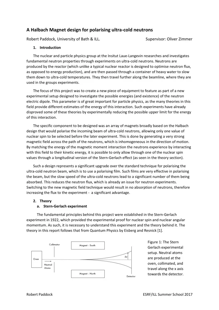
theory in this report follows that from Quantum Physics by Eisberg and Resnick [1]. Figure 1: The Stern Gerlach experimental

• setup. Neutral atoms

are produced at the

• ven, collimated, and

travel along the x axis towards the detector.

Robert Paddock ESRF/ILL Summer School 2017 In this experiment, neutral silver atoms were emitted from an oven and passed through a collimator to produce a beam of neutral atoms, travelling in the +x direction. A transverse magnetic field is applied across a distance a, and a detector is placed a distance b later. This setup can be seen in figure 1. The magnets used to create the field, as seen in figure 2, are specifically designed to create an inhomogeneous field in the z direction. Under a classical physics regime, the neutral beam would not be affected by the magnetic field due to a lack of charge. As such, the beam would continue to travel parallel to the x axis to the detector, producing a single intensity peak. However, the experiment proved this not to be the case, as the magnetic field instead split the beam and two peaks were detected, one either side of the x axis. Instead, the neutral atoms have a magnetic moment that is proportional to the nuclear angular momentum. The energy of such a moment in a magnetic field is given by 𝐹 = 𝜈 ∙ 𝐶, ( 1 ) where 𝜈 is the magnetic moment and B is the applied field. The varying field strength in the z direction therefore causes a force F to act upon the atom which will change its momentum P, 𝐺 = 𝜈𝑨 𝑒𝐶 𝑒𝑨 = 𝑒𝑄

𝑨

𝑒𝑢 , ( 2 ) causing the beam to be deflected away from the z axis. The time ∆𝑢 that each atom experiences the applied field for is a linear function of the distance a and the x component of it’s velocity, ∆𝑢 = 𝑏 𝑊

𝑦

. ( 3 ) This knowledge, along with the mass of the atom being considered, M, means it is possible to calculate the drift velocity ∆𝑊

𝑨 imparted on to the atom by the field,

∆𝑊

𝑨 = ∆𝑄 𝑨

𝑁 = 𝜈𝑨 𝑒𝐶 𝑒𝑨 ∆𝑢 𝑁 = 𝜈𝑨 𝑒𝐶 𝑒𝑨 𝑏 𝑁𝑊

𝑦

. ( 4 ) The time the particle takes to cover distance b and reach the detector after leaving the field is calculated in the same way as seen in equation ( 3 ), which gives an expression for the displacement ∆𝑨 of the beam from the x axis, ∆𝑨 = 𝜈𝑨 𝑒𝐶 𝑒𝑨 𝑏𝑐 𝑁𝑊

𝑦 2.

( 5 ) Figure 2: The magnetic arrangement as seen from the perspective of a neutron travelling along the z direction. The design of the two magnets leads to inhomogeneity of the field in the z direction.

Robert Paddock ESRF/ILL Summer School 2017 Equations ( 2 ) and ( 5 ) show that the force, and the displacement it causes, are proportional to the magnetic moment of the atom being considered. This means that atoms with the different allowed values for nuclear spin, and therefore different magnetic moments, will be deflected by different amounts by the field and thus the beam will be split according to nuclear spin. In our application, we apply instead an inhomogeneous field in the x direction. The reasoning is the same, except that the subsequent force and changes in momentum occur parallel to the direction of the travel of the beam.

• b. The Halbach array

In 1979, Klaus Halbach described an innovative way of arranging recently developed Rare Earth Element permanent magnets to generate a very large magnetic field, for use with particle accelerator beams [2]. The Halbach array features a series of wedge shaped magnets arranged to form a cylinder around a central bore (through which a pipe can be passed). The easy axis of the permanent magnets rotates clockwise around the cylinder, so that the resultant fields of the magnets are aligned in the central bore and so combine to form a very large magnetic field. There are multiple variations of the design depending on the end goal – for example, an easy axis rotation

• f 2π around the circle gives a quadrupole arrangement, while a 4π rotation gives a dipole.

The ideal Halbach array would see a continuous rotation of the easy axis around the central bore, but this obviously cannot be physically represented. In practice, discrete orientations for the easy axis are adequate to generate strong fields, with more used orientations resulting in stronger generated fields. It was shown by Tayler and Sakellariou that this design can also be approximated using small cubic magnets to build a large, square array [3]. Such a design uses only 4 orientations of the easy axis to correspond with the 2D rotational order of 4 of the square magnets – by using only 4

• rientations, the whole design can be created using only one style of magnet. This allows for bulk
• rdering and production, which significantly reduces the cost. This, along with the fact that square

Neodymium magnets as used in this design are readily available for low cost, makes building such an array a feasible prospect. It is also described how such an arrangement can be built in such a way to prevent the individual magnets from moving and potentially being ejected at high speeds from the array. A steel jig is first created, and the magnet positions filled with unmagnetized aluminium blocks. A metal face plate is then attached, which holds the main array in place while providing access to a single block. The magnet corresponding to this position can then be inserted, pushing the metal block out as it

• goes. The face plate is then repositioned to allow access to another block, and the array is

constructed in this fashion.

• 3. Outline of work
• a. Background

A magnetic array was desired to polarise a beam of ultra-cold neutrons, as part of a new experimental setup investigating the electric dipole moment of the neutron. To do this, a longitudinal version of the Stern-Gerlach experiment (explained in section 1a) was applied. The array was designed to generate a very strong magnetic field in the z direction over a small section of pipe, so that as the neutrons approach they see field inhomogeneity in the x direction in the form of a rapidly increasing (and then decreasing) magnetic field. This causes the neutrons to experience a

Robert Paddock ESRF/ILL Summer School 2017 force and thus acceleration in the direction of travel. This acceleration can either increase or decrease the velocity, depending on the spin value of the neutron involved. The applied field was chosen to match the energy of the magnetic moment interaction (expressed in equation 1) with the kinetic energy of the neutrons. The ultra-cold neutrons under consideration have kinetic energies of approximately 90 neV, which corresponds to a magnetic field

• f approximately 1.5T. When a field of this strength is applied, any neutrons with a magnetic

moment opposed to the field will lose all kinetic energy through the interaction with the field, stopping them from travelling any further. Meanwhile, those with magnetic moment aligned to the field will travel on with an increased energy (though this energy will be reduced back to the original value once outside of the influence of the field). This has the effect of polarising the neutron beam, as only neutrons with one specific value of nuclear spin is allowed through. Fields of 1.5T are difficult to obtain, and would typically only be achievable with electromagnets or through utilising supercooling. However, the expense and complexity of this is not very feasible for use in our setup. However, the work of Tayler and Sakellariou demonstrated how a Halbach array can be created using cubic permanent magnets to field strengths similar to this (although over a much smaller bore size, which makes generating strong field substantially easier). This design was of a reasonable size and could be built cheaply (as the magnets required are commonly available). As such, it was decided to attempt to design an array similar to this to polarise the ultra-cold neutrons, using cubic neodymium magnets with 4 orientations. The array would fit around a pipe of 25mm internal radius and 1.5mm thickness, and was required to generate a field of greater than 1.5T across the whole of the inner radius. A high level of homogeneity was also desirable, as this would allow the array to potentially have spectroscopic uses in the future (as it would reduce the range of potential energies that the neutrons passing through would be allowed to have). The design needed to be as small as possible, and as simple as possible (as few magnets/types of magnet as possible) to reduce costs and assembly difficulties.

• b. Criteria

The first part of the project was to simulate the design in 2 dimensions, the decision was made to first consider only 2 dimensions as it reduced the number of variables to initially be considered, resulting in a simpler problem and aiding in become familiar with the software. There were a few key variables that were investigated in 2 dimensions to determine their effects and as such optimal settings. Of these, a key thing to determine was the optimal arrangement of the magnetisation directions around the bore. The Halbach design explains this for a circular array with wedge shaped magnets, but we were trying to approximate this using cubic

• magnets. The Tayler and Sakellariou design had followed the Halbach array quite closely, but it was

possible that a slight deviation from this may work better for cubic magnets, or increase the homogeneity over the Halbach design (which was optimised for field strength only). Some of the other key variables were related to the geometrical shape of the array. The

• riginal Halbach design was a circle, which has equal amounts of magnetic volume assigned to each

Magnetisation orientation. Meanwhile, the Tayler and Sakellariou design, as (roughly) a square, followed the sectioning approach closely, but the nature of the square shape meant some magnetisation directions had a higher volume. It was important to investigate whether a significant advantage would be obtained from making our array more circular (at the expense of increased construction difficulties). Equally, it was important to determine what the bore of the array would

Robert Paddock ESRF/ILL Summer School 2017 look like. The Tayler and Sakellariou design had a rectangular bore (a natural consequence of using

• ne size of square magnets), but the pipe that will pass through the centre of the array was a circle –

this results in wasted volume around the pipe, where the effect of adding magnets is most

• significant. Additionally, the size of a rectangular bore (and a circular bore) is restricted by the size of

the magnets used (as the array needs to fit together, and so the bore must be an integer multiple of the magnet dimension). There were also practical considerations to investigate. It was necessary to find a reasonably sized magnet to use. This was a compromise between two factors – using large magnets meant using less magnets to cover the same volume and would reduce the cost, but would also limit the amount

• f freedom in determining bore size (as discussed earlier). Each magnet can only contain one

magnetisation direction, so it was also important to use one small enough to allow us to simulate the Halbach design effectively (for example, such a design could in theory be made using 4 rectangular magnets only, but at least 8 are required to include any with horizontal magnetisation direction). For this reason, designs using multiple sizes of magnet were also considered. It was also noted that Tayler and Sakellariou used both N48H and N52 magnets in their design, and that this might offer some advantage over just one type of magnet. Finally, it was important to determine the dimensions of the array in total – including length,

• nce the simulations were extended to 3 dimensions). This was essentially a result of the other

variables, as magnets would be added around the outside of the array until the necessary field strength was met. This (along with the simplicity of our design) would act as a measure of success – if the simulations proved such a design to be feasible, then smaller designs would be much favoured, alongside the simplicity to produce and cost.

• c. 2D design - Femm

The 2D simulations were done in a program called Femm, which is available to download for free online [4]. Femm, an acronym for ‘Finite Element Method Magnetics’, uses the Finite Element method to solve some limiting cases of Maxwell’s equations. It can consider both electro and permanent magnets, and addresses ‘low frequency problems’, where any displacement currents can be ignored. The program can be applied to a range of situations – for this project a ‘magnetostatics’ problem was selected, which means that the fields are all time-invariant. The program allows the geometry of the design to be established using simple drawing tools such as lines and arcs. An origin is set and each point is referred to by cartesian coordinates. A grid can also be specified with user-inputted dimensions to aid in the quick construction of designs (without manually selecting the coordinates for each point). Femm also requires boundary conditions to be established. As this problem is an ‘open boundary problem’ the ‘Open boundary builder’ option was used in Femm. This creates a boundary structure to mimic an unbounded domain using Dirichlet edge types over 7 different layers. This was set sufficiently far from the design itself that increasing the distance to the boundary further had no effect. Some brief research was done to get information about what dimensions of cubic magnets are readily available. There is a lot of freedom in this, and a lot of companies offer to produce moulds and then print to custom sizes. 5mm increments in size were common, so it was decided to try and use magnet dimensions that were a multiple of this. It was also discovered that previous work in the Nuclear and Particle Physics group had ordered similar magnets previously, and used N48H magnets.

Robert Paddock ESRF/ILL Summer School 2017 As these were readily available and matched those used by Tayler and Sakellariou, it was decided to use these as the standard. Once the geometry is made in Femm, each region can be selected and its material properties

• defined. The in-built library contains some materials as standard such as air and iron, and other

materials can be defined. For a magnetic material, this requires the use to insert the relative permeability, and the coercive force. For the N48H magnets, permeabilities of 1.05 were used (as recommended by the ‘Femm: Permanent Magnet Example’ [5]. A coercive force of 1059 kA/m was used, as found on the Zhaobao Magnet website (a typical supplier of these magnets) [6]. Some initial designs were drawn to gain familiarity with the program, and to investigate some

• f the variables discussed earlier. The geometries were designed and materials specified, and then

the simulation is run. This produced for each design a plot showing the design and the field lines. The magnetic field can be found at each point, and plots created showing the field change from one point to another. To assess the field across the bore, it was decided that a density plot would be the best thing to use. This allowed the field over the whole of the bore to be seen, which allowed for assessment on inhomogeneity. It also made it easy to identify and measure the point in the bore with the lowest field, which is where the measurement needs to be taken. The magnetisation directions were considered. It was thought that alternative designs (based

• n the Halbach design) may increase the homogeneity across the bore or strengthen the field. For

example, a design around the bore that just uses ‘up’ and ‘down’ orientated magnets may significantly increase the homogeneity, but decrease the field strength. This turned out to be the

• case. However, the ideal Halbach design gave quite poor homogeneity. It was found that the best

compromise was to line the sides of the bore entirely with ‘up’ and ‘down’ magnets, while the corners contained the horizontal directions – this traded roughly 0.1T of field strength from the ideal Halbach design for a very large increase in homogeneity. Each subsequent layer then contained the same number of the ‘up’ and ‘down’ directions, while the numbers of horizontal magnets increased. This is shown in figure 3. This arrangement was selected for the future designs. The effect of adding magnets around the pipe to better fill the space was also investigated. It was found that this significantly increased the magnetic field, but had a negative effect on

• homogeneity. This was because the corners of the magnets typically acted as either a maxima or

minima for field, and by placing a magnet near the pipe the influence of this would be seen. For this reason, increasing the bore size would also increase homogeneity as these corner effects can be reduced – but this again has a large effect on field. Assuming the produced design was sufficiently small, the corner magnets were removed to gain the benefits of increase homogeneity. Figure 3: Such a design was found to offer a good compromise between field strength and

• homogeneity. The sides of the bore

are lined with vertical magnets, while the horizontal magnets are confined to the corners. The second image shows how this design changes as more layers are added.

Robert Paddock ESRF/ILL Summer School 2017 Initial designs that achieved over 1.5T field strengths used 5mm, 10mm and 25mm magnets. This was too complicated for a final design, where ideally just one size was required. It was decided that 20mm magnets were a good solution to attempt to make a design out of. There were sufficiently large that the number of required magnets was relatively low, but small enough that the bore size isn’t too large (with 3 magnets along the bore edge the bore size is 60mm, which will contain the 53mm pipe). This is not too much larger than the pipe itself and would moves the edge magnets relatively far away, which would offer improved homogeneity. There is also the option of adding some corner magnets to increase the field later. Implementing all the findings made above resulted in the Final 2D design seen in figure 4. This design was a very reasonable 260x260mm square, made using only 20x20mm magnets. It generated a field greater than 1.6T across the whole pipe, and was very homogenous with less than 0.1T variation, as seen in figure 5. It would take 160 magnets to produce. As the design was deemed to be of an acceptable size for the experiment and would be sufficiently simple to assemble, it was decided to progress with it to 3 dimensional simulations. Figure 4: The final design from the Femm simulation. Made of 160 20x20mm magnets, the design is a 260x260mm square with a 60x60mm bore to account for the 53mm diameter pipe. No corner magnets are used. The magnetic orientations follow those seen and discussed in figure 3.

Robert Paddock ESRF/ILL Summer School 2017

• d. 2D design – Femm (Tuneable device)

It was also of interest to investigate the feasibility of building a tuneable device. This concept is based on two separate Halbach arrays. An initial, small array would house the pipe as discussed in section 3e, while a larger Halbach array would then be built around this design. The geometry of the two rings would be designed such that there is space to rotate the inner ring inside the outer one. Each array is designed to independently generate a field of 0.8T in the central bore. As such, when the two rings are aligned (i.e., the magnetisation directions on the outer ring are in the same directions as on the inner ring), the field in the centre will sum to the 1.6T required. However, when the rings are opposed (one ring is rotated by 180 degrees relative to the other), the fields will

• ppose one another and the field should drop to effectively zero in the centre. This would allow the

design to be turned on and off, and to generate lower value fields using the same device. A few initial designs were created to better understand the problem. It was important to try and generate a field close to 0.8T on the first ring to have a design that was most efficient in terms of magnets used – if a higher field was generated (as in some of the initial designs), while the 1.6T field is quickly achieved many more magnets must be added before the fields will eventually cancel in the aligned direction. Equally, generating a lower field means that more magnets must be added to try and bring the ‘aligned’ fields up to 1.6T, even though a 0T ‘opposed’ field has already been obtained. This will then continue to decrease the ‘opposed’ field, resulting in a non-zero field in the opposite direction. A design was created, again based on the findings in section 3c, that met the criteria. This design however is much more complicated than the single plate, although efforts have been made to keep the construction and dimensions as simple as possible. The design can be seen in figure 6. It features a central plate with a 60mm bore, but with a 140mm diameter (at the longest point). The inner plate is made of 20x20mm magnets, with additional 20x20mm magnets and some 10x10mm magnets to round off the inner plate. This has been rounded (unlike in section 3c, where a square design was used for simplicity) because just using square shapes results in a large amount of wasted space between the two plates. Figure 5: The contour plot from Femm for the design in figure 4. As can be seen on the legend, the contours represent a field change of 0.25T. The lowest field is 1.65T, with

• nly 3 contours in

the pipe representing an inhomogeneity of 0.75T.

Robert Paddock ESRF/ILL Summer School 2017 The outer plate is made of 25x25mm magnets (although this could be adapted to use 20x20mm magnets is necessary), and is 3 magnets thick at the sides and four at the corners. This array is square, except for a single 25x25mm magnet on each of the inside corners. This produces an

• verall size of 325x325mm for the design. As required, it generates a field that is 1.55T when

aligned, with an inhomogeneity of 0.1T. When opposed, the field is under 0.04T across the whole pipe (sufficiently close to zero for the required purpose). The contour plots can be seen in figure 7 and 8. Figure 6: The tuneable design, from Femm. The inner plate consists

• f 28 20x20mm

magnets and 8 10x10mm magnets, while the outer plate consists of 64 25x25mm magnet. The overall design is 325x325mm. Figure 7: The contour plot from Femm for the two aligned plates. The minimum field strength is 1.55T, at the horizontal edges of the pipe. The four visible contours correspond to an inhomogeneity of 0.1T

Robert Paddock ESRF/ILL Summer School 2017 Such a design adds significant complexity to the problem compared to a single plate, making it much more difficult to assemble as well as to simulate in 3 dimensions. As such, it was decided that the single plate design would be created in 3D instead, and would be the design to be eventually

• constructed. However, this design provided a useful proof of concept (and feasibility) for a tuneable

design, showing it is possible and maintains a reasonable size. If the single plate design is constructed and implemented and found to be successful, it may be of interest to return to this design with the intention of developing it further.

• e. 3D design – Radia

The tuneable design was then simulated in 3 dimensions in a program called Radia [7]. Radia, a program that runs in Wolfram Mathematica, was developed by the European Synchrotron and Radiation Facility dedicated to 3D magnetostatics computations, and is based on boundary Integral methods as opposed to the Finite Element methods seen in FEMM. Radia is also available for free download, although a licence is required for Mathematica. The interface of Radia is very different to Femm. In Femm the geometry of the problem is displayed, which allows the user to clearly see where each point is placed and draw lines between

• them. In Radia, this is not the case – the user must define create objects by defining their

coordinates, and no visual representation of this is displayed unless this is coded in and the code is

• run. This means the coordinates need to be determined beforehand (unlike in Femm, where new

geometries can quickly be created through placing new points on the grid in the correct positions), and it is much less intuitive to build designs. Additionally, as each object must be defined individually it becomes very time consuming to build designs with large numbers of magnets – for this reason, when creating designs in Radia the decision was made to group all magnets with the same magnetisation direction in each region into one larger magnet. This has no effect on the results, and allows the design seen in section 3c. to be built using only 8 objects, as seen in figure 9. Figure 8: The contour plot from Femm for the two

• pposed plates. The

maximum field strength is 0.04T, at the corners of the pipe.

Robert Paddock ESRF/ILL Summer School 2017 There are however advantages to the approach Radia takes to constructing designs. Through the appropriate use of variables in coordinates when building objects, it was possible to make designs that could then quickly and easily be adjusted. For example, bore size and height could be set as parameters, and then when changed the coordinates of the objects would automatically change in response to accommodate this. This means that although the initial construction of the design takes longer, this only needs to be done once – changes are then much easier to make. As in Femm, it was necessary to input the magnetic materials. The material N48H was created for this. Radia needed different information than Femm – it instead wanted the Susceptibility, and the Remanence field. The susceptibility can easily be calculated from the relative permeability, leading to a value of 0.05. A remanence field value of 1.40T was used, again taken the Zhaobao Magnet website. This magnetic property was then applied to each of the created objects. The final design from section 3c was constructed in this fashion, but with a finite length. The strong magnetic field only needs to appear for a short distance – it is essentially a potential barrier, so it doesn’t matter how long it continues for. As such, it was hoped that this could be achieved with a short length. However, the Radia simulations proved that length had a large effect on the generated field strength. While at very long lengths (above 500mm) the contour plot looked identical to that seen in Femm, at shorter lengths (less than 200mm) the field was significantly

• weaker. It was found that to achieve a field strength of above 1.5T, a minimum length of about

200mm was required. The contour plots for different lengths can be seen in figure 10. a) b) Figure 9: The design in Radia (right) was built using only 8 magnetic objects – this is identical to the design in Femm (left), but is much quicker to construct.

Robert Paddock ESRF/ILL Summer School 2017 c) d) 200mm is not an unreasonable length, but any reduction in size corresponds to a reduction in magnetic volume, which would substantially decrease cost and make assembly easier. Additionally, it was also decided that it would be best to have some tolerance in the design to account for the fact that the purchased magnets would not be ideal, and there may be some variance in strength and in magnetisation direction. As such, it would be better to simulate a design with a stronger field so that when built these changes would not reduce the field under 1.5T. It was decided that 1.8T would offer a good solution to this. To decrease the length, the Halbach design was extended to 3 dimensions – this was not something that had been seen in the literature, but required a relatively small change. The regular Halbach design is 2 dimensional, and the magnets serve to focus the magnetic field in the centre of the plane. When extended to 3D this design was merely elongated. However, it is unnecessary to focus the field in the centre of the plane along the whole length of the device, as the strong field is

• nly required in a very thin slice. As such, the device was split into three separate parts – an inner

plate, and an outer plate either side. The inner and outer plates could either be equal in dimensions,

• r different. The magnets in the outer plates were changed slightly from those on the inner plate so

that when a cut through the centre along the length of the design was viewed from the side, it again formed a Halbach array – but focusing the magnetisation in the centre of the length. This was not perfect as the bore passes through where two of the ‘down’ magnets should be, but there should still be enough magnets to have an effect. This concept can be seen in figure 10. Figure 10: The Femm contour plot (a) compared to contour plots in Radia for 200mm (b), 100mm (c), and 20mm (d) lengths. Note the different scales on the plots. While the 200mm plot is essentially the same as seen in Radia, the shorter lengths are very different. Figure 11: The blue inner plate follows the traditional 2D Halbach

• design. This has been placed

between the 2 red outer plates following the new design, to create a 3D Halbach array.

Robert Paddock ESRF/ILL Summer School 2017 This change offered significant improvement in field strength in the centre of the design, which allowed the length to be reduced. A 1.5T field strength could be achieved using this design with a device only 14cm long. While this adds significant complexity to the construction of the device (3 plates must now be independently assembled and fitted together), this is significantly outweighed by the reduction in size (and thus cost). Inserts into the array were again considered. These had been decided against in the Femm designs as it allowed for the production of designs with greater homogeneity. However, it was decided to further investigate them in Radia to see what reduction it would enable in length. 2 sets

• f inserts were considered initially. Trapezium inserts (which allowed the bore to essentially follow

an octagonal shape which would fit closer to the pipe), and ‘full space’ inserts (which were the trapezium inserts with the corner gaps filled in). The ‘full space’ inserts produce a stronger field as they use all the available space, but they require two shapes of magnet as opposed to just one. It’s also worth noting that even the trapezium design cannot be built using just one bulk bought magnet, as the magnetization direction changes relative to the shape. It is worth noting that any shape other than a rectangle is very difficult to make in Radia. For a rectangle, the central coordinate is inserted, along with lengths in the x, y and z directions. For

• ther shapes, this obviously does not work. It is possible to build such shapes by specifying the

vertices of the face, and the length of the object. However, Radia always assumes that the length is along the x axis, and this is not possible to change. The coordinates of the face are then specified in (y, z) form. To obtain a shape with length on the z axis (as was required for this project), the parts must be assembled in this way, and then rotated using the rotation command, where an angle and rotation direction (i.e. +x, -y etc.) are specified. This makes assembling such objects difficult to keep track of – especially when the object is symmetrical such as here, since when the design is viewed it is difficult to determine if the pieces are actually in the correct positions. The final approach for this was to draw the design out with the faces in the x, y plane on paper. The coordinates were then rewritten in (y, x) form. These were then inserted into Radia (with the (y, x) coordinates used when (y, z) coordinates were requested), and a 90-degree rotation around the y axis to translate the z axis

• nto the x axis was applied.

The two styles of insert were tested in a few different combinations – inserts only on the inner plate, inserts on all the plates in the new 3D Halbach orientation, and inserts on all plates in the inner plate orientation throughout the whole design (henceforth referred to as the Extended 2D configuration). It was found that the full space inserts offered significant advantages over the trapezium inserts. For example, when inserted in Femm it offered an increase of 0.1T over the trapezium inserts (although this increase was measured in the centre, and was less extreme at the edges), and a further 0.1T over no inserts at all. It was also found that increasing the size of the inserts increased the field strength. This is thought to be because they followed the Halbach design more closely than the large-scale structure around it. This in theory would reduce the homogeneity – but in practice the transition to the 3D Halbach design had already reduced the homogeneity quite significantly, so this change wasn’t

• noticeable. The rationale behind increasing the insert size was to increase the structural integrity of

these inserts. They were previously quite thin, and it was worried that they would be too at risk of breaking during assembly. To increase the size of these, the first row of 20x20mm magnets was removed, and the inserts increased to fill this space. While the full space inserts were effective, the decision was made to try and approximate this design using rectangular inserts. This was to reduce cost of the magnets – the full space inserts

Robert Paddock ESRF/ILL Summer School 2017 were a very non-standard shape and would add significant cost to the project, so the minor reduction in field strength was worth the saving. To do this, a large square magnet was placed in each corner. Rectangular magnets were then placed along the edges between corners. The full space and rectangular inserts can be seen in figure 12. The increase in field strength from having inserts throughout the whole design as opposed to just the inner plate was significant enough to justify this design. It was also found that while for the small inserts the difference between the 3D Halbach and Extended 2D Halbach designs was unnoticeable, the effect on field strength was large enough when the first row of inner magnets was removed that the Halbach design was selected. An investigation then took place to find the size/shape that used the fewest magnets to achieve the required field strength. A few key parameters were decided upon to do this. Previous experiments had briefly looked at the effect of having unequal heights for the inner and outer plates, as well as unequal lengths – it was found that the freedom that this offered in terms of potential designs did not sufficiently reduce the number of magnets required enough to justify the additional complexity of assembly. It was decided that square magnets of 20x20mm would be used, which meant the height of the array could only increase in 40mm increments. It was decided that these magnets should have integer length, so each layer length could only increase in 10mm increments – this meant the overall length could only increase in 30mm increments. For lengths ranging from 120mm to 240mm, the smallest possible height (that fit our above criteria) was found that produced the desired 1.8T field, and the magnetic volume required to produce this was recorded. These lengths were chosen as the number of magnets for these dimensions seemed to be significantly increased compared to those for the intermediate lengths. Following this process, the optimal dimensions were found to be a height of 260mm, and a length of 240mm. The Tayler and Sakellariou paper used two types of magnets, N48H and N52. The N52 magnets were used for the ‘up’ orientation magnets. It was decided that this should also be investigated for our design to see if It could offer an improvement in field strength (and so a further reduction in size). An investigation of this was undertaken, changing various magnets in the design from N52 ranging from just the inserts on the inner plate to all the up magnets across the whole

• design. This was found to not have a significant impact on field strength, and thus was not worth the

increased complexity and cost associated with it. However, Femm and Radia still showed quite significant inhomogeneity which ideally should be removed. This inhomogeneity was in the form of a stronger field focussed around the corners of Figure 12: The full space inserts on the left were approximated using rectangular inserts, consisting of 4 long rectangles and 4 squares in the corners.

Robert Paddock ESRF/ILL Summer School 2017 the square bore, and a weaker component on the centre of the edges. A variety of combinations of further, smaller inner magnets were attempted to reduce this, which led to a very significant discovery – by placing small magnets in areas of high field strength that were in the opposite direction to that of the conventional Halbach design, the strong magnetic field in that area could be reduced slightly, and would instead increase the field in weaker areas. By using 5mm by 5mm magnets to do this, it was possible to significantly increase the homogeneity. As the magnets are very small compared to the rest of the design, this had a relatively insignificant impact on the overall field strength. This was done on the inner plate only, as extending throughout the whole length so no significant benefit. The new design can be seen in figure 13, and the effects in Femm seen in figure 14. Figure 13: The design in Femm, showing only the inner magnets of the

• design. 8 new magnets have been

added around the corner magnets. 4 of these, which sit adjacent to an ‘up’ magnet, have ‘down’ magnetic

• rientation. The other 4, which sit at

the horizontal sides and fit next to ‘down’ magnets, have an ‘up’

• rientation.

Figure 14: Contour plots from Femm comparing the designs with and without the new opposing magnets. The homogeneity is much increased, for a sacrifice of 0.025T at the strongest point (each contour = 0.025T).

Robert Paddock ESRF/ILL Summer School 2017 In Femm, this resulted in a very homogeneous design. However, while still more homogenous than without the inserts, the results in Radia looked very different. This was shown to be the effects of the 3D Halbach design, and was observed with all the contour plots in Radia and not just the new inserts. When the script was run in Radia for the traditional 2D Halbach design, the results were identical to those in Femm. A comparison of the contour plots for the new design in Femm and Radia can be seen in figure 15, along with a Radia contour plot for the extended 2D design. Adding the new magnets increased the homogeneity, and this had another large effect. The weakest areas of magnetic field strength occur at the edges/corners of the design, where the field changes very quickly. By minimising the size of these areas, this effectively suppressed this effect, increasing the lowest field values experienced in the pipe. This meant that by adding the additional magnets, it was almost possible to reduce the size of the design to 260mmx260mmx210mm – a decrease in required length of 30mm, and so a significant decrease in cost. As can be seen in figure 15, the weakest section in the pipe was at the horizontal edges. As such, efforts were made to reduce the anisotropy in an attempt to reduce this section, and hopefully remove it from the pipe. The idea behind this was to artificially create some anisotropy in the opposite direction, to cancel out the effects of the 3D Halbach design. This meant attempting to create vertical anisotropy in Femm through changes to the newly inserted 5mm by 5mm magnets. This was done by removing the opposed magnets along the vertical edges (the opposed magnets with the ‘down’ orientation) and increasing the length of the down opposed magnet. This had the desired effect in Femm, creating a vertical anisotropy similar to the horizontal one seen in Radia. This was then implemented to the Radia designs. Initially, this magnet was extended to a 5mm by 6mm rectangle. This made the contours in Radia more isotropic and reduced the area at the side that was under 1.8T significantly, but did not quite remove it from the pipe entirely. A 7mm length was then attempted. This further increased the isotropy, and completely removed the section under 1.8T at the sides – unfortunately, it ended a sub Figure 15: The contour plot for the new design in Femm, compared to that for the 3D Halbach design in Radia, and the extended 2D design in Radia. The Extended 2D and Femm designs are essentially identical, showing that the differences in the 3D Halbach design must arise from the 3D Halbach structure (as this is the only difference). The 3D Halbach design demonstrates an anisotropy, with the field much more homogenous along the horizontal axis than across the

• vertical. The circle in the 3D Halbach pipe represents the pipe cross section.

Robert Paddock ESRF/ILL Summer School 2017 1.8T section at the corners so it was just inside the pipe. However, a 6.5mm length for these magnets found a good compromise between the two, excluding both sections from the pipe so that the whole area experienced a field over 1.8T. The final design with 5mm by 6.5mm opposed magnets can be seen in figure 16 and 17 for the Femm and Radia simulations respectively. Figure 16: The final design in Femm, focusing on the inserts only. The four opposed magnets along the vertical edge were removed, and those along the horizontal edge were increased in length so that they are now 5mm by 6.5mm. This creates a vertical anisotropy, that can be seen in the contour plot (scale the same as for all earlier Femm contour plots). Figure 17: The final design in Radia. The contour plot is much more isotropic than previously. The field is greater than 1.8T across the whole pipe area (represented by the circle).

Robert Paddock ESRF/ILL Summer School 2017 .

• f. Future work

The design seen in figures 16 and 17 fulfils all the criteria. Most importantly, it generates a field strength greater than 1.8T across the whole area of the pipe, which is sufficiently strong to polarise the neutron beam, and should account for the fact that real magnets will not be perfect. It is also relatively homogenous, with a range of 0.15T seen across the whole area – a percentage uncertainty of 8.3%. This achieved in a size of 260mm by 260mm by 210mm, which is very reasonable considering the field strength it generates. It has been decided that this device will be built, and magnets are currently being purchased in order to do this. To reduce the complexity of assembly, magnets will be bought that are the whole length of each layer i.e. 7cm. This means that in total 460 magnets are required, which should not generate unreasonable expense. Further work needs to be done on the assembly process. Jigs will obviously be required to assemble the device, but it is also important to consider how the assembly will occur as many powerful magnets are going to be placed in close proximity, and the Tayler and Sakellariou method will not necessarily be appropriate due to the number of magnets. Additionally, further work needs to be done on shielding around the device. A brief investigation was undertaken on the effects of shielding, but a variety of problems were encountered and there was unfortunately not time to solve them all. Of these, the main issue was inputting the material properties for iron in to Radia – this must be done in the same way as a magnetic material (i.e. remanence field and susceptibility), and these properties were not readily available (and may not adequately describe the material).

• 4. Conclusions

A pseudo-Halbach array capable of generating a magnetic field strength of 1.8T across a pipe of radius 25mm was created – the first time such a design has been seen. This was done with an array that measures 260mm by 260mm by 210mm, which is a relatively compact design that should be able to fit easily into the existing setup. The 460 magnets required to build the device will now be

• rdered, and the device assembled.

Two key discoveries were made in the designing of this array, allowing large increases in

• homogeneity. The first was in lining the sides of the bore solely with vertically aligned magnets, and

then placing the horizontal orientations in the corners as the device expanded. More significantly, it was found that placing small magnets in the opposite orientation to the Halbach design in areas of high field strength displaced the field to areas where the strength was lower, significantly reducing the variation in the field. In the development of this design many factors were considered. The end result gave the

• ptimal compromise of these for the required purpose, especially the cost and simplicity of

assembly, the size of the array, the strength of the field, and the homogeneity. The produced field strength exceeded the initial hopes for the design, and the 1.8T produced gives 0.3T tolerance for imperfections in components and assembly.

Robert Paddock ESRF/ILL Summer School 2017

• 5. References

[1] Eisberg, R., Resnick, R. (1985) Quantum Physics of Atoms, Molecules, Solids, Nuclei and Particles, 2nd Edition, New York: Wiley, pp 272 - 275 [2] Halbach, K. (1979) Design of permanent multipole magnets with oriented rare earth Cobalt

• material. Nuclear Instruments and Methods, 169(1), pp 1-10.

[3] Tayler, M.C.D, Sakellariou, D. (2017) Low-cost, pseudo-Halbach dipole magnets for NMR. Journal of Magnetic Resonance, 277, pp 143-148. [4] Meeker, D, (Unknown), Femm [Computer Software]. Retrieved from: http://www.femm.info/wiki/HomePage [5] Meeker, D, (2012), Finite Element Method Magnetics: Permanent Magnet Example [Online]. Available at: http://www.femm.info/wiki/permanentmagnetexample [6] Zhaobao Magnet (Unknown), NdFeB Magnet Magnetic Properties [Online]. Available at: http://www.zhaobao-magnet.com/pro_1.shtml [7] Chubar, O., Elleaume, P., Chavanne, J. (1997), Radia [Computer Software]. Retrieved from: http://www.esrf.eu/Accelerators/Groups/InsertionDevices/Software/Radia