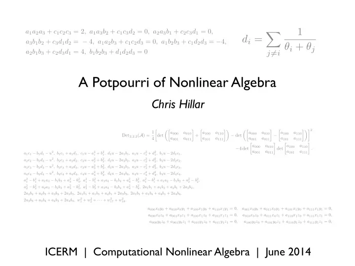

A Potpourri of Nonlinear Algebra
Chris Hillar
ICERM | Computational Nonlinear Algebra | June 2014
di = X
j6=i
1 θi + θj
a1a2a3 + c1c2c3 = 2, a1a3b2 + c1c3d2 = 0, a2a3b1 + c2c3d1 = 0, a3b1b2 + c3d1d2 = − 4, a1a2b3 + c1c2d3 = 0, a1b2b3 + c1d2d3 = −4, a2b1b3 + c2d3d1 = 4, b1b2b3 + d1d2d3 = 0
a1c1 − b1d1 − u2, b1c1 + a1d1, c1u − a2
1 + b2 1, d1u − 2a1b1, a1u − c2 1 + d2 1, b1u − 2d1c1,
a2c2 − b2d2 − u2, b2c2 + a2d2, c2u − a2
2 + b2 2, d2u − 2a2b2, a2u − c2 2 + d2 2, b2u − 2d2c2,
a3c3 − b3d3 − u2, b3c3 + a3d3, c3u − a2
3 + b2 3, d3u − 2a3b3, a3u − c2 3 + d2 3, b3u − 2d3c3,
a4c4 − b4d4 − u2, b4c4 + a4d4, c4u − a2
4 + b2 4, d4u − 2a4b4, a4u − c2 4 + d2 4, b4u − 2d4c4,
a2
1 − b2 1 + a1a3 − b1b3 + a2 3 − b2 3, a2 1 − b2 1 + a1a4 − b1b4 + a2 4 − b2 4, a2 1 − b2 1 + a1a2 − b1b2 + a2 2 − b2 2,
a2
2 − b2 2 + a2a3 − b2b3 + a2 3 − b2 3, a2 3 − b2 3 + a3a4 − b3b4 + a2 4 − b2 4, 2a1b1 + a1b2 + a2b1 + 2a2b2,
2a2b2 + a2b3 + a3b2 + 2a3b3, 2a1b1 + a1b3 + a2b1 + 2a3b3, 2a1b1 + a1b4 + a4b1 + 2a4b4, 2a3b3 + a3b4 + a4b3 + 2a4b4, w2
1 + w2 2 + · · · + w2 17 + w2 18.
Det2,2,2(A) = 1 4 det ✓ a000 a010 a001 a011
- +
a100 a110 a101 a111 ◆ − det ✓ a000 a010 a001 a011
- −
a100 a110 a101 a111 ◆2 −4 det a000 a010 a001 a011
- det
a100 a110 a101 a111
- .
a000x0y0 + a010x0y1 + a100x1y0 + a110x1y1 = 0, a001x0y0 + a011x0y1 + a101x1y0 + a111x1y1 = 0, a000x0z0 + a001x0z1 + a100x1z0 + a101x1z1 = 0, a010x0z0 + a011x0z1 + a110x1z0 + a111x1z1 = 0, a000y0z0 + a001y0z1 + a010y1z0 + a011y1z1 = 0, a100y0z0 + a101y0z1 + a110y1z0 + a111y1z1 = 0,