An Analytical Study of GPU Computation for Solving QAPs by Parallel - - PowerPoint PPT Presentation

an analytical study of gpu computation
SMART_READER_LITE
LIVE PREVIEW

An Analytical Study of GPU Computation for Solving QAPs by Parallel - - PowerPoint PPT Presentation

CEC/CIGPU 201 CEC/CIGPU 2010, 0, Barcelona Barcelona, July 2010 An Analytical Study of GPU Computation for Solving QAPs by Parallel Evolutionary Computation with Independent Run Shigeyoshi Tsutsui Hannan Univ., JAPAN Noriyuki Fujimoto


slide-1
SLIDE 1

CEC/CIGPU 201 CEC/CIGPU 2010, 0, Barcelona Barcelona, July 2010

An Analytical Study of GPU Computation for Solving QAPs by Parallel Evolutionary Computation with Independent Run

Shigeyoshi Tsutsui Hannan Univ., JAPAN Noriyuki Fujimoto Osaka Prefecture Univ., JAPAN

1

slide-2
SLIDE 2

CEC/CIGPU 201 CEC/CIGPU 2010, 0, Barcelona Barcelona, July 2010

Outline of This Talk

  • Background of the research
  • Effect of parallel independent run on GPU
  • Quadratic Assignment Problem (QAP)
  • Implementation Details on GPU
  • Results
  • Analytical study
  • Conclusions and Future Work

2

slide-3
SLIDE 3

CEC/CIGPU 201 CEC/CIGPU 2010, 0, Barcelona Barcelona, July 2010

Background

  • In a previous study (CIGPU 2009), we applied GPU

computation to solve quadratic assignment problems (QAPs) with parallel EC on a single GPU

  • The results in that study showed that parallel EC with the

GTX285 GPU produce a speedup of x3 to x12 compared to the i7 965 (3.2 GHz)

  • However, the analysis of the results was postponed for

future work

  • In this study, we propose a simplified parallel EC model

and analyze how the speedup is obtained using a statistical model of parallel runs of the algorithm

slide-4
SLIDE 4

CEC/CIGPU 201 CEC/CIGPU 2010, 0, Barcelona Barcelona, July 2010

Parallel EC Models

Coarse-grained Model (Distributed EC)

Fine-grained Model Hybrid Model Individual-level Model

Master Slave Slave Slave

Master-Slave Model

slide-5
SLIDE 5

CEC/CIGPU 201 CEC/CIGPU 2010, 0, Barcelona Barcelona, July 2010

Parallel EC Model on GPU

  • Parallel Independent Run Model

– A variant of the coarse-grained model – Gives a lower bound performance of the coarse-grained model – Each sub-population runs on each MP independently – On an MP, individual level parallel run is performed

sub-populations 1 2 p

VRAM (Global Memory) Multi-Processor (30) TP Shared Memory (SM) TP TP TP TP TP TP TP TP Shared Memory (SM) TP TP TP TP TP TP TP TP Shared Memory (SM) TP TP TP TP TP TP TP TP Shared Memory (SM) TP TP TP TP TP TP TP TP Shared Memory (SM) TP TP TP TP TP TP TP TP Shared Memory (SM) TP TP TP TP TP TP TP

slide-6
SLIDE 6

CEC/CIGPU 201 CEC/CIGPU 2010, 0, Barcelona Barcelona, July 2010

Effect of Parallel Independent Run

Run time Tavg Obviously, Tavg>Tp,avg Sequential run Run time Parallel independent run

slide-7
SLIDE 7

CEC/CIGPU 201 CEC/CIGPU 2010, 0, Barcelona Barcelona, July 2010

Quadratic Assignment Problem (QAP)

  • One of the hardest combinatorial optimization

problem

  • Problem size is at most 150
  • Given l locations and l facilities, the task is to assign the

facilities to the locations to minimize the cost

– For each pair of locations i and j, the distance is dij – For each pair of facilities r and s, the flow is frs – The cost is defined as:



 

l i j i l j ijd

f cost

1 ) ( ) ( 1

) (

 

7

slide-8
SLIDE 8

CEC/CIGPU 201 CEC/CIGPU 2010, 0, Barcelona Barcelona, July 2010

location 1 location 2 location 3 location 4 2 5 6 10 4 3 21 facility 1 facility 2 facility 4 facility 3 44 11 30 9 12

an assignment 

1 2 3 4

2 1 4 3

 =

An Example of QAP (l=4)

1524 ) (

4 1 ) ( ) ( 4 1

 

  i j i j ijd

f cost

 

1 2 3 4 1 0

5 10 2

2 5

6 3

3 10

6 4

4 2

3 4

distance matrix d ij location

location

1 2 3 4 1 0

21 11 44

2 21

12 30

3 11 12

9

4 44 30

9

flow matrix f rs facility

facility

8

slide-9
SLIDE 9

CEC/CIGPU 201 CEC/CIGPU 2010, 0, Barcelona Barcelona, July 2010 I1 I2 IN I1 I2 IN '

better Pair wise selection

P W Ii

Apply Crossover and mutation Select another parent randomly

' '

The Base EC Model of a Sub-population

  • We use population pool P and working pool W

9

  • Each individual i (i=1,2,…, N) is processed independently of other

individuals.

  • Re-initialize if number of individuals which have current best functional

value is greater than N*0.6

slide-10
SLIDE 10

CEC/CIGPU 201 CEC/CIGPU 2010, 0, Barcelona Barcelona, July 2010

Implementation Details on GPUs

VRAM constant memory Constant data for QAP(fij, dij) TP TP TP TP TP TP TP TP shared memory(16KB) MP 1 TP TP TP TP TP TP TP TP MP 30 shared memory(16KB)

10

Foundflag=0 Check or set solution was found

Assume problem size at most 56 subpop size N=128 String is array of unsigned char

slide-11
SLIDE 11

CEC/CIGPU 201 CEC/CIGPU 2010, 0, Barcelona Barcelona, July 2010

Experimental Conditions

11

CPU Intel Core i7 965 GPU NVIDIA GeForce GTX285 (240 procs, VRAM 1GB)×2 OS Windows XP Compiler Visual Studio 2005 with /O2 SDK CUDA 2.3 Number of runs 30 Problem instances tai25b, kra30a, kra30b, tai30b, kra32, tai35b, ste36b, tai40b, tai50b from QAPLIB

slide-12
SLIDE 12

CEC/CIGPU 201 CEC/CIGPU 2010, 0, Barcelona Barcelona, July 2010

The run time gain obtained by p-block parallel runs to single block runs

  • The values of gain are different from instance to instance

– They are in the range [10, 35] for p = 30, and [10, 70] for p = 60, – and are nearly proportional to p, except for some instances

10 20 30 40 50 60 70 80

tai25b kra30a kra30b tai30b kra32 tai35b ste36b tai40b tai50b

QAP Instances gain 1GPU (p=30) 2GPUs (p=60)

slide-13
SLIDE 13

CEC/CIGPU 201 CEC/CIGPU 2010, 0, Barcelona Barcelona, July 2010

Sequential run f(t), F(t) g(p,t), G(p,t)

Run Time Estimation of Independent Parallel Run (1)

Parallel independent run p

slide-14
SLIDE 14

CEC/CIGPU 201 CEC/CIGPU 2010, 0, Barcelona Barcelona, July 2010

Run Time Estimation of Independent Parallel Run (2)

dt t f t F p t p M t f t F p t p G dt d t p g t F t p G dt t f t F p

t p p p t t

) ( )) ( 1 ( ) ( ) ( )) ( 1 ( ) , ( ) , ( )) ( 1 ( 1 ) , ( ) ( ) ( blocks run with t independen parallel

  • f

Run time

1 1

            

 

    

 

   ) ( ) 1 ( run block single with Run time

t

dt t f t M

 

    

     

1

) ( )) ( 1 ( ) ( ) ( ) 1 ( blocks run with t independen parallel by

  • btained

Gain

t p t p

dt t f t F p t dt t f t p M M Gain p

slide-15
SLIDE 15

CEC/CIGPU 201 CEC/CIGPU 2010, 0, Barcelona Barcelona, July 2010

Run time distribution on a single block

* * * * * * * * * * * * * * * * * * * * * * * * * * * * * * * * * * * * * * * * * * * * * * * * * * * * * * * * * * * * * * * * * * * * * * * * * * * * * * * * * * * * * * * * * * * * * * * * * * * * * * * * * * * * * * * * * * * * * * * * * * * * * * * * * * * * * * * * * * * * * * * * * * * * * * * * * * * * * * * * * * * * * * * * * * * * * * * * * * * * * * * * * * * * * * * * * * * * * * * * * * * * * * * * * * * * * * * * * * * * * * * * * * * * * * * * * * * * * * * * * * * * * * * * * * * * * * * * * * * * * * * * * * * * * * * * * * * * * * * * * * * * * * * * * * * * * * * * * * * * * * * * * * * * * * * * * * * * * * * * * * * * * * * * * * * * * * * * * * * * * * * * * * * * * * * * * * * * * * * * * * * * * * * * * * * * * * * * * * * * * * * * * * * * * * * * * * * * * * * * * * * * * * * * * * * * * * * * * * * * * * * * * * * * * * * * * * * * * * * * * * * * * * * * * * * * * * * * * * * * * * * * * * * * * * * * * * * * * * * * * * * * * * * * * * * * * * * * * * * * * * * * * * * * * * * * * * * * * * * * * * * * * * * * * * * * * * * * * * * * * * * * * * * * * * * * * * * * * * * * * * * * * * * * * * * * * * * * * * * * * * * * * * * * * * * * * * * * * * * * * * * * * * * * * * * * * * * * * * * * * * * * * * * * * * * * * * * * * * * * * * * * * * * * * * * * * * * * * * * * * * * * * * * * * * * * * * * * * * * * * * * * * * * * * * * * * * * * * * * * * * * * * * * * * * * * * * * * * * * * * * * * * * * * * * * * * * * * * * * * * * * * * * * * * * * * * * * * * * * * * * * * * * * * * * * * * * * * * * * * * * * * * * * * * * * * * * * * * * * * * * * * * * * * * * * * * * * * * * * * * * * * * * * * * * * * * * * * * * * * * * * * * * * * * * * * * * * * * * * * * * * * * * * * * * * * * * * * * * * * * * * * * * * * * * * * * * * * * * * *

tai25b kra30a kra30b tai30b kra32 tai35b ste36b tai40b tai50b 0.1 1 10 100 1000 time (sec) QAP Instances

slide-16
SLIDE 16

CEC/CIGPU 201 CEC/CIGPU 2010, 0, Barcelona Barcelona, July 2010

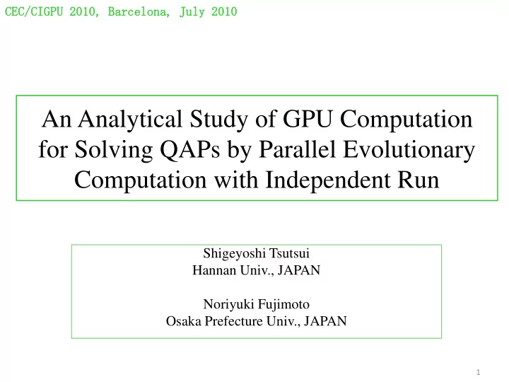
G distribution reflects run time well

50 100 150 200 250 0.0 0.2 0.4 0.6 0.8 1.0 2 4 6 8 10 0.0 0.2 0.4 0.6 0.8 1.0 100 200 300 400 0.0 0.2 0.4 0.6 0.8 1.0 100 200 300 400 0.0 0.2 0.4 0.6 0.8 1.0 100 200 300 400 500 600 700 0.0 0.2 0.4 0.6 0.8 1.0 10 20 30 40 50 60 0.0 0.2 0.4 0.6 0.8 1.0 100 200 300 400 500 600 700 0.0 0.2 0.4 0.6 0.8 1.0 10 20 30 40 50 60 70 0.0 0.2 0.4 0.6 0.8 1.0 200 400 600 800 0.0 0.2 0.4 0.6 0.8 1.0

) 0.607618 exp( 599176 . ) (

.198665

t t t f   ) 0.0381741 exp( 0391455 . ) (

0.00937411

t t t f  

) 0.0124745 exp( 0.01002 ) (

0.056873

t t t f   ) 0.07004 exp( 0.0641907 ) (

0.0412383

t t t f   ) 0.0189536 exp( 0.0187351 ) (

0.0138902

t t t f  

tai25b kra30a kra30b tai30b kra32 tai35b ste36b tai40b tai50b

) 0.0137032 exp( 0.0096430 ) (

0.0928131

t t t f   ) 0167154 . exp( 0.0187351 ) (

0327138 .

t t t f  

) 0697346 . exp( 0.0535232 ) (

0.121357

t t t f  

) 0.00439429 exp( 0.00544967 ) (

.0447259

t t t f  

F(t) t

slide-17
SLIDE 17

CEC/CIGPU 201 CEC/CIGPU 2010, 0, Barcelona Barcelona, July 2010

An example of G distribution

2 4 6 8 10 0.0 0.1 0.2 0.3 0.4

t

tai25b

slide-18
SLIDE 18

CEC/CIGPU 201 CEC/CIGPU 2010, 0, Barcelona Barcelona, July 2010

Comparison between Experimental and Analytical Results

Instances GPU GPU GPU T p,avg M (P )  p T p,avg M (P )  p T p,avg M (P )  p 1 2.02

  • 34.25
  • 113.69
  • 30

0.21 0.03 0.18 1.35 0.79 0.56 3.17 2.92 0.25 GPU2 60 0.19 0.00 0.18 0.70 0.34 0.36 1.63 1.21 0.42 Instances GPU GPU GPU T p,avg M (P )  p T p,avg M (P )  p T p,avg M (P )  p 1 14.31

  • 56.18
  • 92.08
  • 30

0.71 0.45 0.25 2.13 1.78 0.35 3.67 3.25 0.41 GPU2 60 0.46 0.16 0.30 1.12 0.83 0.29 1.65 1.66

  • 0.01

Instances GPU GPU GPU T p,avg M (P )  p T p,avg M (P )  p T p,avg M (P )  p 1 70.82

  • 19.07
  • 212.55
  • 30

2.57 1.63 0.94 1.15 0.46 0.69 8.75 6.19 2.56 GPU2 60 1.35 0.66 0.70 0.90 0.12 0.78 4.28 2.72 1.56 G G tai50b tai40b G G GPU G GPU1 GPU GPU1 GPU kra32 GPU1 No of blocks p tai25b No of blocks p G No of blocks p tai30b ste36b G tai35b G kra30a kra30b G

slide-19
SLIDE 19

CEC/CIGPU 201 CEC/CIGPU 2010, 0, Barcelona Barcelona, July 2010

CPU (T avg )

Population Size

GPU1 GPU2 tai25b 0.21 0.19 0.82 128 3.9 4.4 kra30a 1.35 0.70 6.64 1024 4.9 9.5 kra30b 3.17 1.63 25.20 128 7.9 15.4 tai30b 0.71 0.46 2.05 512 2.9 4.4 kra32 2.13 1.12 10.70 128 5.0 9.5 tai35b 3.67 1.65 12.16 512 3.3 7.4 ste36b 2.57 1.35 15.07 256 5.9 11.1 tai40b 1.15 0.90 4.44 512 3.9 5.0 tai50b 8.75 4.28 18.76 512 2.1 4.4 Values of T 30,avg , T 60,avg and M (P ) are in seconds QAP instances GPU Computaion speedup CPU Computation GPU1 (T 30,avg) GPU2 (T 60,avg)

Comparison between GPU and CPU Computation

19 19

slide-20
SLIDE 20

CEC/CIGPU 201 CEC/CIGPU 2010, 0, Barcelona Barcelona, July 2010

Conclusions

  • We proposed an EA for solving QAPs with parallel independent

runs using GPU computation and gave an analysis of the results

  • In this parallel model, a set of small-size subpopulations was run

in parallel in each block in CUDA independently

  • With this scheme, we got a performance of GPU computation that

is almost proportional to the number of equipped multiprocessors (MPs) in the GPUs

  • We explained these computational results by performing statistical

analysis

  • Regarding performance comparison to CPU computations, GPU

computation showed a speedup of x4.4 and x7.9 on average using a single GPU and two GPUs, respectively

slide-21
SLIDE 21

CEC/CIGPU 201 CEC/CIGPU 2010, 0, Barcelona Barcelona, July 2010

Future Work

  • To obtain higher speedup values, we need to improve

the implementation of variation operator used in each thread in the blocks

  • Each warp of 32 threads is essentially run in a SIMD

fashion in a MP; high performance can only be achieved if all of a warp’s threads execute the same instruction

  • We can consider many parallel evolutionary models

for GPU computation. To implement these models and analyze them remain for future work

slide-22
SLIDE 22

CEC/CIGPU 201 CEC/CIGPU 2010, 0, Barcelona Barcelona, July 2010

kra30a

50 100 150 200 250 300 350 50 100 150 M[1]/ M[p]

slide-23
SLIDE 23

CEC/CIGPU 201 CEC/CIGPU 2010, 0, Barcelona Barcelona, July 2010

tai50b

20 40 60 80 100 120 140 160 180 200 1 10 20 30 40 50 60 70 80 90 100 110 120

slide-24
SLIDE 24

CEC/CIGPU 201 CEC/CIGPU 2010, 0, Barcelona Barcelona, July 2010

tai40b

200 400 600 800 1000 1200 1400 1600 1800 1 10 20 30 40 50 60 70 80 90 100 110 120 系列1

slide-25
SLIDE 25

CEC/CIGPU 201 CEC/CIGPU 2010, 0, Barcelona Barcelona, July 2010

tai35b

20 40 60 80 100 120 140 1 10 20 30 40 50 60 70 80 90 100 110 120

slide-26
SLIDE 26

CEC/CIGPU 201 CEC/CIGPU 2010, 0, Barcelona Barcelona, July 2010

tai30b

50 100 150 200 250 300 350 400 450 1 10 20 30 40 50 60 70 80 90 100 110 120

slide-27
SLIDE 27

CEC/CIGPU 201 CEC/CIGPU 2010, 0, Barcelona Barcelona, July 2010

tai25b

5000 10000 15000 20000 25000 30000 35000 40000 45000 50000 1 10 20 30 40 50 60 70 80 90 100 110 120

slide-28
SLIDE 28

CEC/CIGPU 201 CEC/CIGPU 2010, 0, Barcelona Barcelona, July 2010

ste36b

50 100 150 200 250 300 350 400 1 10 20 30 40 50 60 70 80 90 100 110 120

slide-29
SLIDE 29

CEC/CIGPU 201 CEC/CIGPU 2010, 0, Barcelona Barcelona, July 2010

kra32 20 40 60 80 100 120 140 160 180 1 10 20 30 40 50 60 70 80 90 100 110 120

slide-30
SLIDE 30

CEC/CIGPU 201 CEC/CIGPU 2010, 0, Barcelona Barcelona, July 2010

kra30b 50 100 150 200 250 300 350 1 10 20 30 40 50 60 70 80 90 100 110 120