Analysis of multistate data with thenetsurvival orcause specific - - PDF document

analysis of multistate data with
SMART_READER_LITE
LIVE PREVIEW

Analysis of multistate data with thenetsurvival orcause specific - - PDF document

stick to this world Analysis of multistate data with thenetsurvival orcause specific survival : realistic rate models and t S c ( t ) = exp c ( s ) d s multiple time scales: 0 not a proper probability A


slide-1
SLIDE 1

Analysis of multistate data with realistic rate models and multiple time scales: A dogmatic approach

Bendix Carstensen Steno Diabetes Center Gentofte, Denmark http://BendixCarstensen.com IARC, Lyon, France, 11 April 2018

1/ 51

The dogma [1]

◮ do not condition on the future — indisputable ◮ do not count people after they are dead — disputable ◮ stick to this world — expandable

2/ 51

do not condition on the future

◮ commonly seen in connection with“immortal time bias” ◮ allocation of follow-up (risk time) to a covariate value only

assumed in the future

◮ all follow-up among persons ever on insulin allocated to the

insulin group — including the time prior to insulin use (when not on insulin)

◮ events always with the correct covariate values ◮ ⇒ too much PY in insulin group; rates too small ◮ ⇒ too little PY in non-insulin group; rates too large ◮ ⇒ insulin vs. non-insulin rates underestimated

3/ 51

do not count people after they are dead

◮ Reference to Fine & Gray’s paper on models for the

subdistribution hazard [2]

◮ Recall: hazard and cumulative risk for all cause death:

F(t) = 1−exp

  • −Λ(t)

λ(t) = Λ′(t) =

  • log
  • 1−F(t)

◮ Subdistribution hazard — with more causes of death

(compting risks), for cumulative risk of cause c, Fc(t): ˜ λc(t) =

  • log
  • 1 − Fc(t)

◮ Note: Fc depends on all cause-specific hazards

4/ 51

do not count people after they are dead

◮ The estimation of the subdistribution hazard boils down to:

˜ h(t) = P {X (t + dt) = j|X (t) = j} / dt that is, the instantaneous rate of failure per time unit from cause j among those who are either alive or have died from causes other than j at time t

◮ . . . sounds crazy, but. . . ◮ when modeling the cumulative risk you must refer back to

the size of the original population, which include those dead from other causes.

◮ The debate is rather if the subdistribution hazard is a useful

scale for modeling and reporting from competing risk settings

5/ 51

stick to this world

◮ the“net”survival or“cause specific survival”

: Sc(t) = exp t λc(s) ds

  • ◮ not a proper probability

◮ the probability of survival if

◮ all other causes of death than c were absent ◮ c-specific mortality rate were still the same

◮ so it is just a transformation of the cause-specific rate with no

real world interpretation

◮ . . . do not label quantities“survival”or“probability”when they

are not (of this world)

6/ 51

(further) dogma for “sticking to this world”

◮ rates are continuous in time (and“smooth”

)

◮ rates may depend on more than one time scale ◮ which, is an empirical question

7/ 51

A look at the Cox model

λ(t, x) = λ0(t) × exp(x ′β) A model for the rate as a function of t and x. Covariates:

◮ x ◮ t ◮ . . . often the effect of t is ignored (forgotten?) ◮ i.e. left unreported

8/ 51

The Cox-likelihood as profile likelihood

◮ One parameter per death time to describe the effect of time

(i.e. the chosen timescale). log

  • λ(t, xi)
  • = log
  • λ0(t)
  • + β1x1i + · · · + βpxpi
  • ηi

= αt + ηi

◮ Profile likelihood:

◮ Derive estimates of αt as function of data and βs

— assuming constant rate between death/censoring times

◮ Insert in likelihood, now only a function of data and βs ◮ This turns out to be Cox’s partial likelihood

◮ Cumulative intensity (Λ0(t)) obtained via the

Breslow-estimator

9/ 51

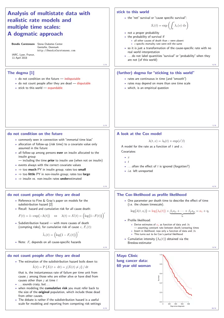
Mayo Clinic lung cancer data: 60 year old woman

200 400 600 800 0.0 0.2 0.4 0.6 0.8 1.0 Days since diagnosis Survival 10/ 51

slide-2
SLIDE 2

Splitting the dataset a priori

◮ The Poisson approach needs a dataset of empirical rates (d, y)

with suitably small values of y.

◮ — each individual contributes many empirical rates ◮ (one per risk-set contribution in Cox-modelling) ◮ From each empirical rate we get:

◮ Poisson-response d ◮ Risk time y → log(y) as offset ◮ time scale covariates: current age, current date, . . . ◮ other covariates

◮ Contributions not independent, but likelihood is a product ◮ Same likelihood as for independent Poisson variates ◮ Poisson glm with spline/factor effect of time

11/ 51

Example: Mayo Clinic lung cancer

◮ Survival after lung cancer ◮ Covariates:

◮ Age at diagnosis ◮ Sex ◮ Time since diagnosis

◮ Cox model ◮ Split data:

◮ Poisson model, time as factor ◮ Poisson model, time as spline 12/ 51

Mayo Clinic lung cancer 60 year old woman

200 400 600 800 0.0 0.2 0.4 0.6 0.8 1.0 Days since diagnosis Survival 13/ 51

Example: Mayo Clinic lung cancer I

> library( survival ) > library( Epi ) > Lung <- Lexis( exit = list( tfe=time ), + exit.status = factor(status,labels=c("Alive","Dead")), + data = lung ) NOTE: entry.status has been set to "Alive" for all. NOTE: entry is assumed to be 0 on the tfe timescale. > summary( Lung ) Transitions: To From Alive Dead Records: Events: Risk time: Persons: Alive 63 165 228 165 69593 228

14/ 51

Example: Mayo Clinic lung cancer II

> system.time( + mL.cox <- coxph( Surv( tfe, tfe+lex.dur, lex.Xst=="Dead" ) ~ + age + factor( sex ), + method="breslow", data=Lung ) ) user system elapsed 0.010 0.001 0.009 > Lung.s <- splitLexis( Lung, + breaks=c(0,sort(unique(Lung$time))), + time.scale="tfe" ) > summary( Lung.s ) Transitions: To From Alive Dead Records: Events: Risk time: Persons: Alive 19857 165 20022 165 69593 228 > subset( Lung.s, lex.id==96 )[,1:11] ; nlevels( factor( Lung.s$tfe ) )

15/ 51

Example: Mayo Clinic lung cancer III

lex.id tfe lex.dur lex.Cst lex.Xst inst time status age sex ph.ecog 9235 96 5 Alive Alive 12 30 2 72 1 2 9236 96 5 6 Alive Alive 12 30 2 72 1 2 9237 96 11 1 Alive Alive 12 30 2 72 1 2 9238 96 12 1 Alive Alive 12 30 2 72 1 2 9239 96 13 2 Alive Alive 12 30 2 72 1 2 9240 96 15 11 Alive Alive 12 30 2 72 1 2 9241 96 26 4 Alive Dead 12 30 2 72 1 2 [1] 186 > system.time( + mLs.pois.fc <- glm( lex.Xst=="Dead" ~ - 1 + factor( tfe ) + + age + factor( sex ), +

  • ffset = log(lex.dur),

+ family=poisson, data=Lung.s, eps=10^-8, maxit=25 ) + ) user system elapsed 13.550 17.334 8.761

16/ 51

Example: Mayo Clinic lung cancer IV

> length( coef(mLs.pois.fc) ) [1] 188 > t.kn <- c(0,25,100,500,1000) > dim( Ns(Lung.s$tfe,knots=t.kn) ) [1] 20022 4 > system.time( + mLs.pois.sp <- glm( lex.Xst=="Dead" ~ Ns( tfe, knots=t.kn ) + + age + factor( sex ), +

  • ffset = log(lex.dur),

+ family=poisson, data=Lung.s, eps=10^-8, maxit=25 ) + ) user system elapsed 0.418 0.510 0.317

17/ 51

Example: Mayo Clinic lung cancer V

> ests <- + rbind( ci.exp(mL.cox), + ci.exp(mLs.pois.fc,subset=c("age","sex")), + ci.exp(mLs.pois.sp,subset=c("age","sex")) ) > cmp <- cbind( ests[c(1,3,5) ,], + ests[c(1,3,5)+1,] ) > rownames( cmp ) <- c("Cox","Poisson-factor","Poisson-spline") > colnames( cmp )[c(1,4)] <- c("age","sex") > round( cmp, 7 ) age 2.5% 97.5% sex 2.5% 97.5% Cox 1.017158 0.9989388 1.035710 0.5989574 0.4313720 0.8316487 Poisson-factor 1.017158 0.9989388 1.035710 0.5989574 0.4313720 0.8316487 Poisson-spline 1.016189 0.9980329 1.034676 0.5998287 0.4319932 0.8328707

18/ 51 200 400 600 800 0.1 0.2 0.5 1.0 2.0 5.0 10.0 Days since diagnosis Mortality rate per year 200 400 600 800 0.0 0.2 0.4 0.6 0.8 1.0 Days since diagnosis Survival 19/ 51 200 400 600 800 2 4 6 8 10 Days since diagnosis Mortality rate per year 200 400 600 800 0.0 0.2 0.4 0.6 0.8 1.0 Days since diagnosis Survival 19/ 51

slide-3
SLIDE 3

Deriving the survival function

> mLs.pois.sp <- glm( lex.Xst=="Dead" ~ Ns( tfe, knots=t.kn ) + + age + factor( sex ), +

  • ffset = log(lex.dur),

+ family=poisson, data=Lung.s, eps=10^-8, maxit=25 ) > CM <- cbind( 1, Ns( seq(10,1000,10)-5, knots=t.kn ), 60, 1 ) > lambda <- ci.exp( mLs.pois.sp, ctr.mat=CM ) > Lambda <- ci.cum( mLs.pois.sp, ctr.mat=CM, intl=10 )[,-4] > survP <- exp(-rbind(0,Lambda))

Code and output for the entire example available in http://bendixcarstensen.com/AdvCoh/WNtCMa/

20/ 51

What the Cox-model really is

Taking the life-table approach ad absurdum by:

◮ dividing time very finely and ◮ modeling one covariate, the time-scale, with one parameter per

distinct value.

◮ the model for the time scale is really with exchangeable

time-intervals.

◮ ⇒ difficult to access the baseline hazard (which looks terrible) ◮ ⇒ uninitiated tempted to show survival curves where irrelevant

21/ 51

Models of this world

◮ Replace the αts by a parametric function f (t) with a limited

number of parameters, for example:

◮ Piecewise constant ◮ Splines (linear, quadratic or cubic) ◮ Fractional polynomials

◮ the two latter brings model into“this world”

:

◮ smoothly varying rates ◮ parametric closed form representation of baseline hazard ◮ finite no. of parameters

◮ Makes it really easy to use rates directly in calculations of

◮ expected residual life time ◮ state occupancy probabilities in multistate models ◮ . . . 22/ 51

additional dogma

Not sacred, merely consequenecs of the 3rd commandment:

◮ Show risk time in states and transitions between states

graphically

◮ Model transition rates by smooth parametric functions ◮ There is no such thing as primary or secondary time scale —

time scales and other quantitative covariates should be modeled the same way

◮ Determine the relevant timescale(s) ◮ Then derive the relevant measures to report. ◮ Time-scale interactions is the proper name for

“non-proportional hazards”

◮ Multiple time scales should be reported jointly

23/ 51

EBMT transplant data

Iacobelli & Carstensen: Multistate Models with Multiple Timescales, Stat Med 2013, [3]

Trans 30,504.1 Relap 6,106.5 Dead(Tr) Dead(Relap) 2,246 (7.4) 3,683 (12.1) 1,076 (17.6) Trans 30,504.1 Relap 6,106.5 Dead(Tr) Dead(Relap) Trans 30,504.1 Relap 6,106.5 Dead(Tr) Dead(Relap)

µT(t) µR(t, r, tR) λ(t)

  • ther covariates: Age and date at Tx, sex, donor type, CML type

24/ 51 1980 1990 2000 10 20 30 40 50 60 70 Date Age

  • 1980

1990 2000 10 20 30 40 50 60 70 Date Time since Transplant

  • ● ●
  • ●● ●
  • ● ●
  • ●● ●
  • 5

10 15 20 25 10 20 30 40 50 60 70 Time since Relapse Time since Transplant

  • 25/ 51

Markov property: Empirical question

Model for mortality rates:

◮ t time since transplant ◮ r time since relapse (if relapsed) ◮ tr time from transplant to relapse ◮ Fit the model for all transitions:

◮ split follow-up time ◮ fit Poisson model with covariates ◮ and spline terms for each time scale.

◮ Lexis machinery [4, 5] from the Epi package for R ◮ . . . for representation and manipulation of follow-up data.

26/ 51

log(µ) = h(t)+k(r)+g(t − r) + X β

2 4 6 8 10 5 10 20 50 100 200 500 Time since transplant Mortality rate per 1000 PY 2 4 6 8 10 0.2 0.5 1.0 2.0 5.0 10.0 20.0 Time since relapse Mortality rate ratio relapsed at 1 year vs. non−relapsed 2 4 6 8 10 0.2 0.5 1.0 2.0 5.0 10.0 20.0 Time from transplant to relapse Mortality rate ratio

t: time since transplant r: time since relapse

27/ 51

log(µ) = h(t)+k(r)+g(t − r) + X β

1 2 3 4 5 6 7 5 10 20 50 100 200 500 1000 2000 Time since transplant Mortality rate per 1000 PY No relapse Relapse times: 0.17 0.5 1 2 3 4 5 1 2 3 4 5 6 7 5 10 20 50 100 200 500 1000 2000 Time since relapse Mortality rate per 1000 PY Relapse times: 0.17 0.5 1 2 3 4 5

t: time since transplant r: time since relapse

28/ 51

log(µ) = h(t)+k(r)+g(t − r) + X β

1 2 3 4 5 6 7 5 10 20 50 100 200 500 1000 2000 Time since transplant Mortality rate per 1000 PY No relapse Relapse times: 0.17 0.5 1 2 3 4 5 1 2 3 4 5 6 7 5 10 20 50 100 200 500 1000 2000 Time since relapse Mortality rate per 1000 PY Relapse times: 0.17 0.5 1 2 3 4 5

t: time since transplant r: time since relapse

29/ 51

slide-4
SLIDE 4

log(µ) = h(t)+k(r)+g(t − r) + X β

1 2 3 4 5 6 7 5 10 20 50 100 200 500 1000 2000 Time since transplant Mortality rate per 1000 PY No relapse Relapse times: 0.17 0.5 1 2 3 4 5 1 2 3 4 5 6 7 5 10 20 50 100 200 500 1000 2000 Time since relapse Mortality rate per 1000 PY Relapse times: 0.17 0.5 1 2 3 4 5

t: time since transplant r: time since relapse

30/ 51

ARTICLE

Years of life gained by multifactorial intervention in patients with type 2 diabetes mellitus and microalbuminuria: 21 years follow-up on the Steno-2 randomised trial

Peter Gæde1,2 & Jens Oellgaard1,2,3 & Bendix Carstensen3 & Peter Rossing3,4,5 & Henrik Lund-Andersen3,5,6 & Hans-Henrik Parving5,7 & Oluf Pedersen8

Received: 7 April 2016 /Accepted: 1 July 2016 # The Author(s) 2016. This article is published with open access at Springerlink.com

Abstract Aims/hypothesis The aim of this work was to study the poten- tial long-term impact of a 7.8 years intensified, multifactorial pharmacological approaches. After 7.8 years the study contin- ued as an observational follow-up with all patients receiving treatment as for the original intensive-therapy group. The pri-

Diabetologia DOI 10.1007/s00125-016-4065-6

31/ 51 DM 1,108.2 80 28 1st CVD 132.3 5 2nd CVD 44.7 5 3+ CVD 24.7 4 D(no CVD) 17 D(1 CVD) 13 D(2 CVD) 5 D(3+ CVD) 3 35 (3.2) 17 (1.5) 17 (12.9) 13 (9.8) 7 (15.7) 5 (11.2) 3 (12.1) DM 1,108.2 80 28 1st CVD 132.3 5 2nd CVD 44.7 5 3+ CVD 24.7 4 D(no CVD) 17 D(1 CVD) 13 D(2 CVD) 5 D(3+ CVD) 3 DM 1,108.2 80 28 1st CVD 132.3 5 2nd CVD 44.7 5 3+ CVD 24.7 4 D(no CVD) 17 D(1 CVD) 13 D(2 CVD) 5 D(3+ CVD) 3 Intensive DM 762.5 80 13 1st CVD 210.3 6 2nd CVD 67.6 2 3+ CVD 67.4 4 D(no CVD) 16 D(1 CVD) 14 D(2 CVD) 11 D(3+ CVD) 14 51 (6.7) 16 (2.1) 31 (14.7) 14 (6.7) 17 (25.2) 11 (16.3) 14 (20.8) DM 762.5 80 13 1st CVD 210.3 6 2nd CVD 67.6 2 3+ CVD 67.4 4 D(no CVD) 16 D(1 CVD) 14 D(2 CVD) 11 D(3+ CVD) 14 DM 762.5 80 13 1st CVD 210.3 6 2nd CVD 67.6 2 3+ CVD 67.4 4 D(no CVD) 16 D(1 CVD) 14 D(2 CVD) 11 D(3+ CVD) 14 Conventional 32/ 51

DM 1,108.2 80 28 1st CVD 132.3 5 2nd CVD 44.7 D(no CVD) 17 D(1 CVD) 13 D(2 CVD) 5 35 (3.2) 17 (1.5) 17 (12.9) 13 (9.8) 5 (11.2) DM 1,108.2 80 28 1st CVD 132.3 5 2nd CVD 44.7 D(no CVD) 17 D(1 CVD) 13 D(2 CVD) 5 DM 1,108.2 80 28 1st CVD 132.3 5 2nd CVD 44.7 D(no CVD) 17 D(1 CVD) 13 D(2 CVD) 5 Intensive DM 762.5 80 13 1st CVD 210.3 6 2nd CVD 67.6 D(no CVD) 16 D(1 CVD) 14 D(2 CVD) 11 51 (6.7) 16 (2.1) 31 (14.7) 14 (6.7) 11 (16.3) DM 762.5 80 13 1st CVD 210.3 6 2nd CVD 67.6 D(no CVD) 16 D(1 CVD) 14 D(2 CVD) 11 DM 762.5 80 13 1st CVD 210.3 6 2nd CVD 67.6 D(no CVD) 16 D(1 CVD) 14 D(2 CVD) 11 Conventional

33/ 51

Models used

◮ One model for the 4 mortality rates ◮ One model for the 3 CVD rates ◮ . . . both models assume:

◮ proportional hazards between CVD states (0, 1, 2(, 3) CVD events) ◮ proportional hazards between groups (conventional, intervention) ◮ proportional hazards between levels of sex and age (at entry)

◮ Which just means: multiplicative effects of the covariates:

time since baseline, CVD state, group, sex and age

◮ Proportional hazards means:

no interaction with the time scale

34/ 51

Hazard ratios

Mortality CVD event HR, Int. vs. Conv. 0.83 (0.54; 1.30) 0.55 (0.39;0.77) H0: PH btw. CVD groups p=0.438 p=0.261 H0: HR = 1 p=0.425 p=0.001 HR vs. 0 CVD events: 0 (ref.) 1.00 1.00 1 3.08 (1.82; 5.19) 2.43 (1.67;3.52) 2 4.42 (2.36; 8.29) 3.48 (2.15;5.64) 3+ 7.76 (4.11;14.65) Then use fitted rates to estimate the probabilities of being in each state at all times. (This is immensely complicated).

35/ 51 5 10 15 20 0.0 0.2 0.4 0.6 0.8 1.0 Probability 0.0 0.2 0.4 0.6 0.8 1.0 Intensive 20 15 10 5 Conventional Time since baseline (years) 36/ 51

between groups (HR 0.83 [95% CI 0.54, 1.30], p=0.43). Thus, the reduced mortality was primarily due to reduced risk of CVD. The patients in the intensive group experienced a total of 90 cardiovascular events vs 195 events in the conventional

  • group. Nineteen intensive-group patients (24%) vs 34

conventional-group patients (43%) experienced more than

  • ne cardiovascular event. No significant between-group dif-

ference in the distribution of specific cardiovascular first- event types was observed (Table 2 and Fig. 4). Microvascular complications Hazard rates of progression rates in microvascular complications compared with baseline status are shown Fig. 3. Sensitivity analyses showed a negli- gible effect of the random dates imputation. Progression of retinopathy was decreased by 33% in the intensive-therapy group (Fig. 5). Blindness in at least one eye was reduced in the intensive-therapy group with an HR of 0.47 (95% CI 0.23, 0.98, p=0.044). Autonomic neuropathy was decreased by 41% in the intensive-therapy group (Fig. 5). We

  • bserved no difference between groups in the progression of

peripheral neuropathy (Fig. 5). Progression to diabetic ne- phropathy (macroalbuminuria) was reduced by 48% in the intensive-therapy group (Fig. 5). Ten patients in the conventional-therapy groups vs five patients in the intensive- therapy group progressed to end-stage renal disease (p=0.061). Discussion

a

25 50 75 100 Cumulative mortality (%) 80 78 65 45 34 24 Conventional 80 76 66 58 54 43 Intensive Number at risk 4 8 12 16 20 Years since randomisation

b

25 50 75 100 Death or CVD event (%) 80 61 40 27 18 13 Conventional 80 66 56 49 41 31 Intensive Number at risk 4 8 12 16 20 Years since randomisation

37/ 51 5 10 15 20 0.0 0.2 0.4 0.6 0.8 1.0 Probability 0.0 0.2 0.4 0.6 0.8 1.0 Intensive 20 15 10 5 Conventional Time since baseline (years)

Same treatment effects for Death resp. CVD between CVD levels

38/ 51 5 10 15 20 0.0 0.2 0.4 0.6 0.8 1.0 Probability 0.0 0.2 0.4 0.6 0.8 1.0 Intensive 20 15 10 5 Conventional Time since baseline (years)

Different treatment effects for Death resp. CVD between CVD levels

39/ 51

slide-5
SLIDE 5

Expected lifetime and YLL (well, gained)

◮ Expected lifetime (years) in the Steno 2 cohort during the first

20 years after baseline by treatment group and CVD status. State where Int. Conv. Int.−Conv. Alive under black line 15.6 14.1 1.5 No CVD green area 12.7 10.0 2.6 Any CVD

  • range area

3.0 4.1 −1.1

◮ What does“expected”mean? ◮ Expectation w.r.t.

age and sex-distribution in the Steno2 study!

◮ Computed as areas under survival curves

40/ 51

Intensive

0.2 0.4 0.6 0.8 1.0

Conventional

0.2 0.4 0.6 0.8 1.0

Intensive Conventional 45

0.2 0.4 0.6 0.8 1.0 0.2 0.4 0.6 0.8 1.0 0.2 0.4 0.6 0.8 1.0

50

0.2 0.4 0.6 0.8 1.0 0.2 0.4 0.6 0.8 1.0 0.2 0.4 0.6 0.8 1.0

55

0.2 0.4 0.6 0.8 1.0 0.2 0.4 0.6 0.8 1.0 0.2 0.4 0.6 0.8 1.0

60

0.2 0.4 0.6 0.8 1.0 0.2 0.4 0.6 0.8 1.0 5 10 15 20 0.0 0.0 20 15 10 5 0.0 0.2 0.4 0.6 0.8 1.0 5 10 15 20 0.0

65

20 15 10 5 0.0 0.2 0.4 0.6 0.8 1.0

Time since entry (years) Probability Men Women Age

41/ 51

Intensive

0.2 0.4 0.6 0.8 1.0

Conventional

0.2 0.4 0.6 0.8 1.0

Intensive Conventional 45

0.2 0.4 0.6 0.8 1.0 0.2 0.4 0.6 0.8 1.0 0.2 0.4 0.6 0.8 1.0

50

0.2 0.4 0.6 0.8 1.0 0.8 1.0 0.8 1.0 0.8 1.0

Probability Men Women Age

42/ 51

Expected lifetime (years) during the first 20 years after baseline by sex, age, treatment group and CVD status. sex Men Women state age Int. Conv. Int.−Conv. Int. Conv. Int.−Conv. Alive 45 18.5 17.5 1.0 19.1 18.4 0.7 50 17.2 16.1 1.1 18.0 17.2 0.8 55 15.6 13.8 1.8 17.4 15.9 1.6 60 13.9 11.6 2.2 15.5 13.7 1.8 65 11.2 9.5 1.8 13.3 11.4 2.0 No CVD 45 14.9 12.5 2.4 15.8 14.3 1.5 50 14.0 11.1 2.9 15.1 12.9 2.2 55 12.2 9.7 2.5 14.3 11.6 2.7 60 10.9 8.2 2.7 12.4 9.9 2.6 65 9.0 6.7 2.2 10.7 8.3 2.4

43/ 51

Multistate models in practice:

◮ Representation:

◮ States ◮ Transitions ◮ Sojourn times ◮ Rates

◮ Analysis of rates:

◮ Cox-model ◮ Poisson model

◮ Reporting

◮ Rates ◮ HRs ◮ Probabilities ◮ Expected lifetime DM 1,108.2 80 28 1st CVD 132.3 5 2nd CVD 44.7 5 3+ CVD 24.7 4 D(no CVD) 17 D(1 CVD) 13 D(2 CVD) 5 D(3+ CVD) 3 35 (3.2) 17 (1.5) 17 (12.9) 13 (9.8) 7 (15.7) 5 (11.2) 3 (12.1) DM 1,108.2 80 28 1st CVD 132.3 5 2nd CVD 44.7 5 3+ CVD 24.7 4 D(no CVD) 17 D(1 CVD) 13 D(2 CVD) 5 D(3+ CVD) 3 DM 1,108.2 80 28 1st CVD 132.3 5 2nd CVD 44.7 5 3+ CVD 24.7 4 D(no CVD) 17 D(1 CVD) 13 D(2 CVD) 5 D(3+ CVD) 3 Intensive DM 762.5 80 13 1st CVD 210.3 6 2nd CVD 67.6 2 3+ CVD 67.4 4 D(no CVD) 16 D(1 CVD) 14 D(2 CVD) 11 D(3+ CVD) 14 51 (6.7) 16 (2.1) 31 (14.7) 14 (6.7) 17 (25.2) 11 (16.3) 14 (20.8) DM 762.5 80 13 1st CVD 210.3 6 2nd CVD 67.6 2 3+ CVD 67.4 4 D(no CVD) 16 D(1 CVD) 14 D(2 CVD) 11 D(3+ CVD) 14 DM 762.5 80 13 1st CVD 210.3 6 2nd CVD 67.6 2 3+ CVD 67.4 4 D(no CVD) 16 D(1 CVD) 14 D(2 CVD) 11 D(3+ CVD) 14 Conventional 44/ 51

From rates to probabilities

◮ There is a one-to-one correspondence between:

◮ all rates between states (by time) + initial state distribution ◮ state distribution by time

◮ Model for rates

⇒ probability of being in a given state at any given time

◮ Analytically this is a nightmare ◮ Simulation is the answer

45/ 51

From rates to probabilities: simLexis

◮ Assume a person is in“DM”initially

◮ Simulate a time of death (transition to“D(no CVD)”

)

◮ Simulate a time of CVD (transition to“1st CVD”

)

◮ Choose the smaller as the transition

◮ If transition is to“1st CVD”simulate death / 2nd CVD, etc. ◮ Repeat for, say, 10,000 persons

⇒ simulated cohort study

◮ simLexis does this for you, provided you have

◮ initial state and covariates for all persons ◮ models to predict (cumulative) rates

◮ Count how many is in each state at each time:

⇒ state occupancy probabilities

◮ nState and pState does this for you

46/ 51 5 10 15 20 0.0 0.2 0.4 0.6 0.8 1.0 Probability 0.0 0.2 0.4 0.6 0.8 1.0 Intensive 20 15 10 5 Conventional Time since baseline (years) 47/ 51

Using the Lexis machinery

◮ Allows estimation of fully parametric rate function ◮ Simple test for proportional hazards ◮ State occupancy probabilities requires simulation:

simLexis — see vignette in Epi package

◮ Access to other measures such as expected residual lifetime. ◮ — similar machinery available in Stata:

◮ multistate ◮ Crowther & Lambert [6] ◮ Only one timescale, however. . . 48/ 51

Additional dogma

◮ Show risk time in states and transitions between states ◮ Model transition rates by smooth parametric functions ◮ There is no such thing as primary or secondary time scale —

time scales and other quantitative covariates should be modeled the same way

◮ Time-scale interactions is the proper name for

“non-proportional hazards”

◮ Multiple time scales should be reported jointly

49/ 51

slide-6
SLIDE 6

References I

  • P. K. Andersen and N. Keiding.

Interpretability and importance of functionals in competing risks and multistate models. Stat Med, 31:1074–1088, 2012. J P Fine and R J Gray. A proportional hazards model for the subdistribution of a competing risk. Journal of the American Statistical Association, 94(446), 1999.

  • S. Iacobelli and B. Carstensen.

Multiple time scales in multi-state models. Stat Med, 32(30):5315–5327, Dec 2013. Martyn Plummer and Bendix Carstensen. Lexis: An R class for epidemiological studies with long-term follow-up. Journal of Statistical Software, 38(5):1–12, 1 2011. Bendix Carstensen and Martyn Plummer. Using Lexis objects for multi-state models in R. Journal of Statistical Software, 38(6):1–18, 1 2011.

References II

  • M. J. Crowther and P. C. Lambert.

Parametric multistate survival models: Flexible modelling allowing transition-specific distributions with application to estimating clinically useful measures of effect differences. Stat Med, 36(29):4719–4742, Dec 2017.

bendixcarstensen.com/AdvCoh/Lexis-ex