Announcements Reminders: Assignment 1 due Sept 22 11:59 pm on - - PDF document

SLIDE 1

9/19/2017 1

Recognizing object categories

Kristen Grauman UT-Austin Wed Sept 13, 2017

Announcements

• Reminders:
• Assignment 1 due Sept 22 11:59 pm on Canvas
• No laptops, phones, tablets, etc. in class
• Thoughts on review sharing?
• Questions about presentations, experiments,

discussion proponent/opponent?

Last time: Recognizing instances Last time: Recognizing instances

• 1. Basics in feature extraction: filtering
• 2. Invariant local features
• 3. Recognizing object instances

Instance recognition: remaining issues

• How to summarize the content of an entire

image? And gauge overall similarity?

• How large should the vocabulary be? How to

perform quantization efficiently?

• Is having the same set of visual words enough to

identify the object/scene? How to verify spatial agreement?

Kristen Grauman

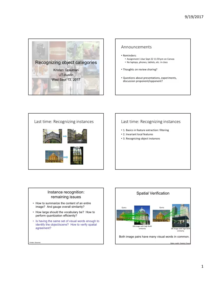
Spatial Verification

Both image pairs have many visual words in common.

Slide credit: Ondrej Chum Query Query DB image with high BoW similarity DB image with high BoW similarity

SLIDE 2

9/19/2017 2

Only some of the matches are mutually consistent

Slide credit: Ondrej Chum

Spatial Verification

Query Query DB image with high BoW similarity DB image with high BoW similarity

Spatial Verification: two basic strategies

• RANSAC
• Generalized Hough Transform

Slide credit: Kristen Grauman

Outliers affect least squares fit Outliers affect least squares fit RANSAC

• RANdom Sample Consensus
• Approach: we want to avoid the impact of outliers,

so let’s look for “inliers”, and use those only.

• Intuition: if an outlier is chosen to compute the

current fit, then the resulting line won’t have much support from rest of the points.

RANSAC for line fitting

Repeat N times:

• Draw s points uniformly at random
• Fit line to these s points
• Find inliers to this line among the remaining

points (i.e., points whose distance from the line is less than t)

• If there are d or more inliers, accept the line

and refit using all inliers

Lana Lazebnik

SLIDE 3

9/19/2017 3

RANSAC for line fitting example

Source: R. Raguram

Lana Lazebnik

RANSAC for line fitting example

Least-squares fit

Source: R. Raguram

Lana Lazebnik

RANSAC for line fitting example

• 1. Randomly select

minimal subset

• f points

Source: R. Raguram

Lana Lazebnik

RANSAC for line fitting example

• 1. Randomly select

minimal subset

• f points
• 2. Hypothesize a

model

Source: R. Raguram

Lana Lazebnik

RANSAC for line fitting example

• 1. Randomly select

minimal subset

• f points
• 2. Hypothesize a

model

• 3. Compute error

function

Source: R. Raguram

Lana Lazebnik

RANSAC for line fitting example

• 1. Randomly select

minimal subset

• f points
• 2. Hypothesize a

model

• 3. Compute error

function

• 4. Select points

consistent with model

Source: R. Raguram

Lana Lazebnik

SLIDE 4

9/19/2017 4

RANSAC for line fitting example

• 1. Randomly select

minimal subset

• f points
• 2. Hypothesize a

model

• 3. Compute error

function

• 4. Select points

consistent with model

• 5. Repeat

hypothesize-and- verify loop

Source: R. Raguram

Lana Lazebnik 24

RANSAC for line fitting example

• 1. Randomly select

minimal subset

• f points
• 2. Hypothesize a

model

• 3. Compute error

function

• 4. Select points

consistent with model

• 5. Repeat

hypothesize-and- verify loop

Source: R. Raguram

Lana Lazebnik 25

RANSAC for line fitting example

• 1. Randomly select

minimal subset

• f points
• 2. Hypothesize a

model

• 3. Compute error

function

• 4. Select points

consistent with model

• 5. Repeat

hypothesize-and- verify loop

Uncontaminated sample

Source: R. Raguram

Lana Lazebnik

RANSAC for line fitting example

• 1. Randomly select

minimal subset

• f points
• 2. Hypothesize a

model

• 3. Compute error

function

• 4. Select points

consistent with model

• 5. Repeat

hypothesize-and- verify loop

Source: R. Raguram

Lana Lazebnik

That is an example fitting a model (line)… What about fitting a transformation (translation, affine…)?

Robust feature-based alignment

Source: L. Lazebnik

SLIDE 5

9/19/2017 5

• Extract features

Source: L. Lazebnik

Robust feature-based alignment

• Extract features
• Compute putative matches

Source: L. Lazebnik

Robust feature-based alignment

• Extract features
• Compute putative matches
• Loop:
• Hypothesize transformation T (small group of putative

matches that are related by T)

Source: L. Lazebnik

Robust feature-based alignment

• Extract features
• Compute putative matches
• Loop:
• Hypothesize transformation T (small group of putative

matches that are related by T)

• Verify transformation (search for other matches consistent

with T)

Source: L. Lazebnik

Robust feature-based alignment

• Extract features
• Compute putative matches
• Loop:
• Hypothesize transformation T (small group of putative

matches that are related by T)

• Verify transformation (search for other matches consistent

with T)

Source: L. Lazebnik

Robust feature-based alignment

RANSAC: General form

• RANSAC loop:

1. Randomly select a seed group of points on which to base transformation estimate 2. Compute model from seed group 3. Find inliers to this transformation 4. If the number of inliers is sufficiently large, re-compute estimate of model on all of the inliers

• Keep the model with the largest number of inliers

SLIDE 6

9/19/2017 6

RANSAC example: Translation

Putative matches

Source: Rick Szeliski

RANSAC example: Translation

Select one match, count inliers

RANSAC example: Translation

Select one match, count inliers

RANSAC example: Translation

Find “average” translation vector

RANSAC verification

For matching specific scenes/objects, common to use an affine transformation for spatial verification

Fitting an affine transformation

) , (

i i y

x   ) , (

i i y

x

                           

2 1 4 3 2 1

t t y x m m m m y x

i i i i

                                                  

i i i i i i

y x t t m m m m y x y x

2 1 4 3 2 1

1 1 Approximates viewpoint changes for roughly planar objects and roughly orthographic cameras.

SLIDE 7

9/19/2017 7

RANSAC verification

Spatial Verification: two basic strategies

• RANSAC

– Typically sort by BoW similarity as initial filter – Verify by checking support (inliers) for possible affine transformations

• e.g., “success” if find an affine transformation with > N inlier

correspondences

• Generalized Hough Transform

– Let each matched feature cast a vote on location, scale, orientation of the model object – Verify parameters with enough votes

Kristen Grauman

Spatial Verification: two basic strategies

• RANSAC

– Typically sort by BoW similarity as initial filter – Verify by checking support (inliers) for possible affine transformations

• e.g., “success” if find an affine transformation with > N inlier

correspondences

• Generalized Hough Transform

– Let each matched feature cast a vote on location, scale, orientation of the model object – Verify parameters with enough votes

Kristen Grauman

Voting

• It’s not feasible to check all combinations of features by

fitting a model to each possible subset.

• Voting is a general technique where we let the features

vote for all models that are compatible with it.

– Cycle through features, cast votes for model parameters. – Look for model parameters that receive a lot of votes.

• Noise & clutter features will cast votes too, but typically

their votes should be inconsistent with the majority of “good” features.

Kristen Grauman

Difficulty of line fitting

Kristen Grauman

Hough Transform for line fitting

• Given points that belong to a line, what

is the line?

• How many lines are there?
• Which points belong to which lines?
• Hough Transform is a voting

technique that can be used to answer all of these questions. Main idea:

• 1. Record vote for each possible line
• n which each edge point lies.
• 2. Look for lines that get many votes.

Kristen Grauman

SLIDE 8

9/19/2017 8

Finding lines in an image: Hough space

Connection between image (x,y) and Hough (m,b) spaces

• A line in the image corresponds to a point in Hough space
• To go from image space to Hough space:

– given a set of points (x,y), find all (m,b) such that y = mx + b

x y m b m0 b0

image space Hough (parameter) space

Slide credit: Steve Seitz

Finding lines in an image: Hough space

Connection between image (x,y) and Hough (m,b) spaces

• A line in the image corresponds to a point in Hough space
• To go from image space to Hough space:

– given a set of points (x,y), find all (m,b) such that y = mx + b

• What does a point (x0, y0) in the image space map to?

x y m b

image space Hough (parameter) space

– Answer: the solutions of b = -x0m + y0 – this is a line in Hough space

x0 y0

Slide credit: Steve Seitz

Finding lines in an image: Hough space

What are the line parameters for the line that contains both (x0, y0) and (x1, y1)?

• It is the intersection of the lines b = –x0m + y0 and

b = –x1m + y1 x y m b

image space Hough (parameter) space

x0 y0

b = –x1m + y1 (x0, y0) (x1, y1)

Finding lines in an image: Hough algorithm

How can we use this to find the most likely parameters (m,b) for the most prominent line in the image space?

• Let each edge point in image space vote for a set of

possible parameters in Hough space

• Accumulate votes in discrete set of bins; parameters with

the most votes indicate line in image space.

x y m b

image space Hough (parameter) space

Voting: Generalized Hough Transform

• If we use scale, rotation, and translation invariant local

features, then each feature match gives an alignment hypothesis (for scale, translation, and orientation of model in image).

Model Novel image

Adapted from Lana Lazebnik

Voting: Generalized Hough Transform

• A hypothesis generated by a single match may be

unreliable,

• So let each match vote for a hypothesis in Hough space

Model Novel image

SLIDE 9

9/19/2017 9

Gen Hough Transform details (Lowe’s system)

• Training phase: For each model feature, record 2D

location, scale, and orientation of model (relative to normalized feature frame)

• Test phase: Let each match btwn a test SIFT feature

and a model feature vote in a 4D Hough space

• Use broad bin sizes of 30 degrees for orientation, a factor of

2 for scale, and 0.25 times image size for location

• Vote for two closest bins in each dimension
• Find all bins with at least three votes and perform

geometric verification

• Estimate least squares affine transformation
• Search for additional features that agree with the alignment

David G. Lowe. "Distinctive image features from scale-invariant keypoints.” IJCV 60 (2), pp. 91-110, 2004.

Slide credit: Lana Lazebnik

Objects recognized, Recognition in spite of occlusion

Example result

Background subtract for model boundaries

[Lowe]

Gen Hough vs RANSAC

GHT

• Single correspondence ->

vote for all consistent parameters

• Represents uncertainty in the

model parameter space

• Linear complexity in number
• f correspondences and

number of voting cells; beyond 4D vote space impractical

• Can handle high outlier ratio

RANSAC

• Minimal subset of

correspondences to estimate model -> count inliers

• Represents uncertainty

in image space

• Must search all data

points to check for inliers each iteration

• Scales better to high-d

parameter spaces

Kristen Grauman

Perceptual and Sensory Augmented Computing Visual Object Recognition Tutorial

Video Google System

• 1. Collect all words within

query region

• 2. Inverted file index to find

relevant frames

• 3. Compare word counts
• 4. Spatial verification

Sivic & Zisserman, ICCV 2003

• Demo online at :

http://www.robots.ox.ac.uk/~vgg/r esearch/vgoogle/index.html

Query region Retrieved frames

Recognition via feature matching+spatial verification

Pros:

• Effective when we are able to find reliable features

within clutter

• Great results for matching specific instances

Cons:

• Scaling with number of models
• Spatial verification as post-processing – not

seamless, expensive for large-scale problems

• Not suited for category recognition.

Kristen Grauman

SLIDE 10

9/19/2017 10

Summary: instance recognition

• Matching local invariant features

– Useful not only to provide matches for multi-view geometry, but also to find objects and scenes.

• Bag of words representation: quantize feature space to

make discrete set of visual words – Summarize image by distribution of words – Index individual words

• Inverted index: pre-compute index to enable faster

search at query time

• [today] Recognition of instances via alignment:

matching local features followed by spatial verification – Robust fitting : RANSAC, GHT

Kristen Grauman

Rest of today

• Intro to categorization problem
• Object categorization as discriminative classification

a) Boosting + fast face detection example b) Nearest neighbors + scene recognition example c) Support vector machines + pedestrian detection example

i. Pyramid match kernels, spatial pyramid match

d) Convolutional neural networks + ImageNet example

What does recognition involve?

Slide credit: Fei-Fei Li

Detection: are there people?

Slide credit: Fei-Fei Li

Activity: What are they doing?

Slide credit: Fei-Fei Li

Object categorization

mountain building tree banner vendor people street lamp

Slide credit: Fei-Fei Li

SLIDE 11

9/19/2017 11

Instance recognition

Potala Palace A particular sign

Slide credit: Fei-Fei Li

Scene and context categorization

• outdoor
• city
• …

Slide credit: Fei-Fei Li

Attribute recognition

flat gray made of fabric crowded

Slide credit: Fei-Fei Li Perceptual and Sensory Augmented Computing Visual Object Recognition Tutorial

• K. Grauman, B. Leibe
• K. Grauman, B. Leibe

Object Categorization

• Task Description
• “Given a small number of training images of a category,

recognize a-priori unknown instances of that category and assign the correct category label.”

• Which categories are feasible visually?

German shepherd animal dog living being “Fido” Perceptual and Sensory Augmented Computing Visual Object Recognition Tutorial

• K. Grauman, B. Leibe
• K. Grauman, B. Leibe

Visual Object Categories

• Basic Level Categories in human categorization

[Rosch 76, Lakoff 87]

• The highest level at which category members have similar

perceived shape

• The highest level at which a single mental image reflects the

entire category

• The level at which human subjects are usually fastest at

identifying category members

• The first level named and understood by children
• The highest level at which a person uses similar motor actions

for interaction with category members

Perceptual and Sensory Augmented Computing Visual Object Recognition Tutorial

• K. Grauman, B. Leibe
• K. Grauman, B. Leibe

Visual Object Categories

• Basic-level categories in humans seem to be defined

predominantly visually.

• There is evidence that humans (usually)

start with basic-level categorization before doing identification.

 Basic-level categorization is easier and faster for humans than object identification!

 How does this transfer to automatic

classification algorithms?

Basic level Individual level Abstract levels “Fido”

dog animal quadruped German shepherd Doberman cat cow … … … … … …

SLIDE 12

9/19/2017 12

How many object categories are there?

Biederman 1987

Source: Fei-Fei Li, Rob Fergus, Antonio Torralba.

Perceptual and Sensory Augmented Computing Visual Object Recognition Tutorial

• K. Grauman, B. Leibe
• K. Grauman, B. Leibe

Other Types of Categories

• Functional Categories
• e.g. chairs = “something you can sit on”

Challenges: robustness

Illumination Object pose Clutter Viewpoint Intra-class appearance Occlusions

Challenges: context and human experience

Context cues

Challenges: context and human experience

Context cues Function Dynamics

Video credit: J. Davis

SLIDE 13

9/19/2017 13 Challenges: complexity

• Millions of pixels in an image
• 30,000 human recognizable object categories
• 30+ degrees of freedom in the pose of articulated
• bjects (humans)
• Billions of images online
• 300 hours of new video on YouTube per minute
• …
• About half of the cerebral cortex in primates is

devoted to processing visual information [Felleman and van Essen 1991]

Challenges: learning with minimal supervision More

Less

Slide from Pietro Perona, 2004 Object Recognition workshop Slide from Pietro Perona, 2004 Object Recognition workshop

Recognizing flat, textured

• bjects (like books, CD

covers, posters) Reading license plates, zip codes, checks Fingerprint recognition Frontal face detection

What kinds of things work best today? What kinds of things work best today?

SLIDE 14

9/19/2017 14

Evolution of methods

• Hand-crafted models
• 3D geometry
• Hypothesize and align
• Hand-crafted features
• Learned models
• Data-driven
• “End-to-end”

learning of features and models*,**

* Labeled data availability ** Architecture design decisions, parameters.

Generic category recognition: basic framework

• Build/train object model

– (Choose a representation) – Learn or fit parameters of model / classifier

• Generate candidates in new image
• Score the candidates

Window-based models Generating and scoring candidates

Car/non-car Classifier

Kristen Grauman

Window-based object detection

Car/non-car Classifier Feature extraction

Training examples Training: 1. Obtain training data 2. Select/learn features/classifier Given new image: 1. Slide window 2. Score by classifier

Kristen Grauman

Object proposals: all windows -> probable regions

How “object-like” is each candidate region?

Constrained Parametric Min-Cuts for Automatic Object Segmentation. Carreira and Sminchisescu. CVPR 2010

Also see Uijlings et al. 2012, Ferrari et al CVPR 2010, Endres et al ECCV 2010

Object recognition as classification

• What classifier?

– Factors in choosing:

• Generative or discriminative model?
• Data resources – how much training data?
• How is the labeled data prepared?
• Training time allowance
• Test time requirements – real-time?
• Fit with the representation

Kristen Grauman

SLIDE 15

9/19/2017 15

Discriminative classifies

106 examples

Nearest neighbor Shakhnarovich, Viola, Darrell 2003 Berg, Berg, Malik 2005, Hays 2008, Torralba 2008,…... Neural networks LeCun, Bottou, Bengio, Haffner 1998 Rowley, Baluja, Kanade 1998, Krizhevsky 2012… … Support Vector Machines Conditional Random Fields McCallum, Freitag, Pereira 2000; Kumar, Hebert 2003 … Guyon, Vapnik Heisele, Serre, Poggio, 2001, Lazebnik 2006…

Slide adapted from Antonio Torralba

Boosting Viola, Jones 2001, Torralba et al. 2004, Opelt et al. 2006,…

Kristen Grauman

• What categories are amenable to window-

based classification?

– Similar to specific object matching, we expect spatial layout to be roughly preserved. – Unlike specific object matching, by training classifiers we attempt to capture intra-class variation

• r determine required discriminative features.

Kristen Grauman

Object recognition as classification

Image classification Three landmark case studies

SVM + person detection

e.g., Dalal & Triggs

Boosting + face detection

Viola & Jones

NN + scene Gist classification

e.g., Hays & Efros

Main idea:

– Represent local texture with efficiently computable “rectangular” features within window of interest – Select discriminative features to be weak classifiers – Use boosted combination of them as final classifier – Form a cascade of such classifiers, rejecting clear negatives quickly

Viola-Jones face detector

Kristen Grauman

Boosting intuition

Weak Classifier 1

Slide credit: Paul Viola

Boosting illustration

Weights Increased

SLIDE 16

9/19/2017 16

Boosting illustration

Weak Classifier 2

Boosting illustration

Weights Increased

Boosting illustration

Weak Classifier 3

Boosting illustration

Final classifier is a combination of weak classifiers

Boosting: training

• Initially, weight each training example equally
• In each boosting round:

– Find the weak learner that achieves the lowest weighted training error – Raise weights of training examples misclassified by current weak learner

• Compute final classifier as linear combination of all weak

learners (weight of each learner is directly proportional to its accuracy)

• Exact formulas for re-weighting and combining weak

learners depend on the particular boosting scheme (e.g., AdaBoost)

Slide credit: Lana Lazebnik

Boosting: pros and cons

• Advantages of boosting
• Integrates classification with feature selection
• Complexity of training is linear in the number of training

examples

• Flexibility in the choice of weak learners, boosting scheme
• Testing is fast
• Easy to implement
• Disadvantages
• Needs many training examples
• Often found not to work as well as an alternative

discriminative classifier, support vector machine (SVM), or CNNs

– especially for many-class problems

Slide credit: Lana Lazebnik

SLIDE 17

9/19/2017 17

Viola-Jones detector: features

Feature output is difference between adjacent regions Efficiently computable with integral image: any sum can be computed in constant time. “Rectangular” filters

Value at (x,y) is sum of pixels above and to the left of (x,y)

Integral image

Kristen Grauman

Computing sum within a rectangle

• Let A,B,C,D be the

values of the integral image at the corners of a rectangle

• Then the sum of original

image values within the rectangle can be computed as:

sum = A – B – C + D

• Only 3 additions are

required for any size of rectangle!

D B C A

Lana Lazebnik

Viola-Jones detector: features

Feature output is difference between adjacent regions Efficiently computable with integral image: any sum can be computed in constant time Avoid scaling images  scale features directly for same cost “Rectangular” filters

Value at (x,y) is sum of pixels above and to the left of (x,y)

Integral image

Kristen Grauman

Considering all possible filter parameters: position, scale, and type: 180,000+ possible features associated with each 24 x 24 window

Which subset of these features should we use to determine if a window has a face? Use AdaBoost both to select the informative features and to form the classifier

Viola-Jones detector: features

Kristen Grauman

Viola-Jones detector: AdaBoost

• Want to select the single rectangle feature and threshold

that best separates positive (faces) and negative (non- faces) training examples, in terms of weighted error.

Outputs of a possible rectangle feature on faces and non-faces.

… Resulting weak classifier: For next round, reweight the examples according to errors, choose another filter/threshold combo.

Kristen Grauman Perceptual and Sensory Augmented Computing Visual Object Recognition Tutorial Visual Object Recognition Tutorial

First two features selected

Viola-Jones Face Detector: Results

SLIDE 18

9/19/2017 18

• Even if the filters are fast to compute, each new

image has a lot of possible windows to search.

• How to make the detection more efficient?

Cascading classifiers for detection

• Form a cascade with low false negative rates early on
• Apply less accurate but faster classifiers first to immediately

discard windows that clearly appear to be negative

Kristen Grauman

Viola-Jones detector: summary

Train with 5K positives, 350M negatives Real-time detector using 38 layer cascade 6061 features in all layers

[Implementation available in OpenCV: http://www.intel.com/technology/computing/opencv/]

Faces Non-faces

Train cascade of classifiers with AdaBoost

Selected features, thresholds, and weights New image

Kristen Grauman

Viola-Jones detector: summary

• A seminal approach to real-time object detection
• Training is slow, but detection is very fast
• Key ideas
• Integral images for fast feature evaluation
• Boosting for feature selection
• Attentional cascade of classifiers for fast rejection of non-

face windows

• P. Viola and M. Jones. Rapid object detection using a boosted cascade of simple features.

CVPR 2001.

• P. Viola and M. Jones. Robust real-time face detection. IJCV 57(2), 2004.

Perceptual and Sensory Augmented Computing Visual Object Recognition Tutorial Visual Object Recognition Tutorial

Viola-Jones Face Detector: Results

Perceptual and Sensory Augmented Computing Visual Object Recognition Tutorial Visual Object Recognition Tutorial

Viola-Jones Face Detector: Results

SLIDE 19

9/19/2017 19

Perceptual and Sensory Augmented Computing Visual Object Recognition Tutorial Visual Object Recognition Tutorial

Viola-Jones Face Detector: Results

Perceptual and Sensory Augmented Computing Visual Object Recognition Tutorial Visual Object Recognition Tutorial

Detecting profile faces?

Can we use the same detector?

Perceptual and Sensory Augmented Computing Visual Object Recognition Tutorial Visual Object Recognition Tutorial

Paul Viola, ICCV tutorial

Viola-Jones Face Detector: Results

Everingham, M., Sivic, J. and Zisserman, A. "Hello! My name is... Buffy" - Automatic naming of characters in TV video, BMVC 2006. http://www.robots.ox.ac.uk/~vgg/research/nface/index.html

Example using Viola-Jones detector

Frontal faces detected and then tracked, character names inferred with alignment of script and subtitles.

Consumer application: iPhoto

http://www.apple.com/ilife/iphoto/

Slide credit: Lana Lazebnik

SLIDE 20

9/19/2017 20

Consumer application: iPhoto

Things iPhoto thinks are faces

Slide credit: Lana Lazebnik

Consumer application: iPhoto

Can be trained to recognize pets!

http://www.maclife.com/article/news/iphotos_faces_recognizes_cats

Slide credit: Lana Lazebnik

Privacy Gift Shop – CV Dazzle

http://www.wired.com/2015/06/facebook-can-recognize-even-dont-show-face/ Wired, June 15, 2015

Slide credit: Kristen Grauman

Privacy Visor

http://www.3ders.org/articles/20150812-japan-3d-printed-privacy-visors- will-block-facial-recognition-software.html

Slide credit: Kristen Grauman

Perceptual and Sensory Augmented Computing Visual Object Recognition Tutorial Visual Object Recognition Tutorial

Window-based detection: strengths

• Sliding window detection and global appearance

descriptors:

• Simple detection protocol to implement
• Good feature choices critical
• Past successes for certain classes

Perceptual and Sensory Augmented Computing Visual Object Recognition Tutorial Visual Object Recognition Tutorial

Window-based detection: Limitations

• High computational complexity
• For example: 250,000 locations x 30 orientations x 4 scales =

30,000,000 evaluations!

• If training binary detectors independently, means cost increases

linearly with number of classes

• With so many windows, false positive rate better be low

SLIDE 21

9/19/2017 21

Perceptual and Sensory Augmented Computing Visual Object Recognition Tutorial Visual Object Recognition Tutorial

Limitations (continued)

• Not all objects are “box” shaped

Perceptual and Sensory Augmented Computing Visual Object Recognition Tutorial Visual Object Recognition Tutorial

Limitations (continued)

• Non-rigid, deformable objects not captured well with

representations assuming a fixed 2d structure; or must assume fixed viewpoint

• Objects with less-regular textures not captured well

with holistic appearance-based descriptions

Perceptual and Sensory Augmented Computing Visual Object Recognition Tutorial Visual Object Recognition Tutorial

Limitations (continued)

• If considering windows in isolation, context is lost

Figure credit: Derek Hoiem

Sliding window Detector’s view

Perceptual and Sensory Augmented Computing Visual Object Recognition Tutorial Visual Object Recognition Tutorial

Limitations (continued)

• In practice, often entails large, cropped training set

(expensive)

• Requiring good match to a global appearance description

can lead to sensitivity to partial occlusions

Image credit: Adam, Rivlin, & Shimshoni

Image classification: Three landmark case studies

SVM + person detection

e.g., Dalal & Triggs

Boosting + face detection

Viola & Jones

NN + scene Gist classification

e.g., Hays & Efros

Slide credit: Kristen Grauman

Nearest Neighbor classification

• Assign label of nearest training data point to each

test data point

Voronoi partitioning of feature space for 2-category 2D data

from Duda et al.

Black = negative Red = positive Novel test example Closest to a positive example from the training set, so classify it as positive.

SLIDE 22

9/19/2017 22

K-Nearest Neighbors classification

k = 5

Source: D. Lowe

• For a new point, find the k closest points from training data
• Labels of the k points “vote” to classify

If query lands here, the 5 NN consist of 3 negatives and 2 positives, so we classify it as negative. Black = negative Red = positive

80M Tiny Images [Torralba et al. 2008]

Where in the World?

[Hays and Efros. im2gps: Estimating Geographic Information from a Single Image. CVPR 2008.]

Where in the World?

Slide credit: James Hays

Where in the World?

Slide credit: James Hays

6+ million geotagged photos by 109,788 photographers

Annotated by Flickr users

Slide credit: James Hays

SLIDE 23

9/19/2017 23

6+ million geotagged photos by 109,788 photographers

Annotated by Flickr users

Slide credit: James Hays

Which scene properties are relevant?

A scene is a single surface that can be represented by global (statistical) descriptors

Spatial Envelope Theory of Scene Representation

Oliva & Torralba (2001)

Slide Credit: Aude Olivia

Global texture: capturing the “Gist” of the scene

Oliva & Torralba IJCV 2001, Torralba et al. CVPR 2003

Capture global image properties while keeping some spatial information

Gist descriptor

Which scene properties are relevant?

• Gist scene descriptor
• Color Histograms - L*A*B* 4x14x14 histograms
• Texton Histograms – 512 entry, filter bank based
• Line Features – Histograms of straight line stats

Scene Matches

[Hays and Efros. im2gps: Estimating Geographic Information from a Single Image. CVPR 2008.] Slide credit: James Hays

SLIDE 24

9/19/2017 24

Slide credit: James Hays

Scene Matches

[Hays and Efros. im2gps: Estimating Geographic Information from a Single Image. CVPR 2008.] Slide credit: James Hays [Hays and Efros. im2gps: Estimating Geographic Information from a Single Image. CVPR 2008.] Slide credit: James Hays

Scene Matches

[Hays and Efros. im2gps: Estimating Geographic Information from a Single Image. CVPR 2008.] Slide credit: James Hays [Hays and Efros. im2gps: Estimating Geographic Information from a Single Image. CVPR 2008.] Slide credit: James Hays

The Importance of Data

[Hays and Efros. im2gps: Estimating Geographic Information from a Single Image. CVPR 2008.]

Slide credit: James Hays

SLIDE 25

9/19/2017 25 Nearest neighbors: pros and cons

• Pros:

– Simple to implement – Flexible to feature / distance choices – Naturally handles multi-class cases – Can do well in practice with enough representative data

• Cons:

– Large search problem to find nearest neighbors – Storage of data – Must know we have a meaningful distance function

Kristen Grauman

Today

• Intro to categorization problem
• Object categorization as discriminative classification
• Boosting + fast face detection example
• Nearest neighbors + scene recognition example
• Support vector machines + pedestrian detection example
• Pyramid match kernels, spatial pyramid match
• Convolutional neural networks + ImageNet example

Image classification: Three landmark case studies

SVM + person detection

e.g., Dalal & Triggs

Boosting + face detection

Viola & Jones

NN + scene Gist classification

e.g., Hays & Efros

Linear classifiers Linear classifiers

• Find linear function to separate positive and

negative examples

: negative : positive       b b

i i i i

w x x w x x Which line is best?

Support Vector Machines (SVMs)

• Discriminative

classifier based on

• ptimal separating

hyperplane

• Maximize the margin

between the positive and negative training examples

SLIDE 26

9/19/2017 26

Support vector machines

• Want line that maximizes the margin.

1 : 1) ( negative 1 : 1) ( positive           b y b y

i i i i i i

w x x w x x

Margin Support vectors

• C. Burges, A Tutorial on Support Vector Machines for Pattern Recognition, Data Mining

and Knowledge Discovery, 1998

For support, vectors,

1     b

i w

x

Support vector machines

• Want line that maximizes the margin.

1 : 1) ( negative 1 : 1) ( positive           b y b y

i i i i i i

w x x w x x

Margin M Support vectors For support, vectors,

1     b

i w

x

Distance between point and line:

|| || | | w w x b

i

  w w w 2 1 1     M

w w x w 1   b

Τ

For support vectors:

Support vector machines

• Want line that maximizes the margin.

1 : 1) ( negative 1 : 1) ( positive           b y b y

i i i i i i

w x x w x x

Support vectors For support, vectors,

1     b

i w

x

Distance between point and line:

|| || | | w w x b

i

 

Therefore, the margin is 2 / ||w|| Margin M

Finding the maximum margin line

• 1. Maximize margin 2/||w||
• 2. Correctly classify all training data points:

Quadratic optimization problem: Minimize Subject to yi(w·xi+b) ≥ 1

w wT 2 1

1 : 1) ( negative 1 : 1) ( positive           b y b y

i i i i i i

w x x w x x

Finding the maximum margin line

• Solution:





i i i i y x

w 

Support vector learned weight

Finding the maximum margin line

• Solution:

b = yi – w·xi (for any support vector)

• Classification function:





i i i i y x

w 

b y b

i i i i

    



x x x w 

• C. Burges, A Tutorial on Support Vector Machines for Pattern Recognition, Data Mining and Knowledge Discovery, 1998

 

b y x f

i i

     



x x x w

i i

sign b) ( sign ) ( 

SLIDE 27

9/19/2017 27

Dalal & Triggs, CVPR 2005

• Map each grid cell in the

input window to a histogram counting the gradients per

• rientation.
• Train a linear SVM using

training set of pedestrian vs. non-pedestrian windows.

Code available: http://pascal.inrialpes.fr/soft/olt/

Person detection with HoG’s & linear SVM’s HoG descriptor

Code available: http://pascal.inrialpes.fr/soft/olt/

Dalal & Triggs, CVPR 2005

Person detection with HoGs & linear SVMs

• Histograms of Oriented Gradients for Human Detection, Navneet Dalal, Bill Triggs,

International Conference on Computer Vision & Pattern Recognition - June 2005

• http://lear.inrialpes.fr/pubs/2005/DT05/

YOLO detector

• https://pjreddie.com/darknet/yolo/

Question

• What if the data is not linearly separable?

Non-linear SVMs

 Datasets that are linearly separable with some noise

work out great:

 But what are we going to do if the dataset is just too hard?  How about… mapping data to a higher-dimensional

space:

x x x x2

SLIDE 28

9/19/2017 28

Nonlinear SVMs

• The kernel trick: instead of explicitly computing

the lifting transformation φ(x), define a kernel function K such that K(xi,xj

j) = φ(xi ) · φ(xj)

• This gives a nonlinear decision boundary in the
• riginal feature space:

b K y

i i i i





) , ( x x 

Example

2-dimensional vectors x=[x1 x2]; let K(xi,xj)=(1 + xi

Txj)2

Need to show that K(xi,xj)= φ(xi) Tφ(xj): K(xi,xj)=(1 + xi

Txj)2 ,

= 1+ xi1

2xj1 2 + 2 xi1xj1 xi2xj2+ xi2 2xj2 2 + 2xi1xj1 + 2xi2xj2

= [1 xi1

2 √2 xi1xi2 xi2 2 √2xi1 √2xi2]T

[1 xj1

2 √2 xj1xj2 xj2 2 √2xj1 √2xj2]

= φ(xi) Tφ(xj), where φ(x) = [1 x1

2 √2 x1x2 x2 2 √2x1 √2x2]

Examples of kernel functions

 Linear:

 Gaussian RBF:  Histogram intersection:

) 2 exp( ) (

2 2



j i j i

x x ,x x K   





k j i j i

k x k x x x K )) ( ), ( min( ) , (

j T i j i

x x x x K  ) , (

SVMs for recognition

• 1. Define your representation for each

example.

• 2. Select a kernel function.
• 3. Compute pairwise kernel values

between labeled examples

• 4. Use this “kernel matrix” to solve for

SVM support vectors & weights.

• 5. To classify a new example: compute

kernel values between new input and support vectors, apply weights, check sign of output.

Kristen Grauman

Local feature correspondence useful similarity measure for generic object categories

Kristen Grauman

What about a matching kernel?

Partially matching sets of features

We introduce an approximate matching kernel that makes it practical to compare large sets of features based on their partial correspondences.

Optimal match: O(m3) Greedy match: O(m2 log m) Pyramid match: O(m)

(m=num pts)

[Previous work: Indyk & Thaper, Bartal, Charikar, Agarwal & Varadarajan, …]

Kristen Grauman

SLIDE 29

9/19/2017 29 Pyramid match: main idea

descriptor space

Feature space partitions serve to “match” the local descriptors within successively wider regions.

Kristen Grauman

Pyramid match: main idea

Histogram intersection counts number of possible matches at a given partitioning.

Kristen Grauman

Pyramid match kernel

• For similarity, weights inversely proportional to bin size

(or may be learned)

• Normalize these kernel values to avoid favoring large sets

[Grauman & Darrell, ICCV 2005]

measures difficulty of a match at level number of newly matched pairs at level

Pyramid match kernel

• ptimal partial

matching

Optimal match: O(m3) Pyramid match: O(mL)

Kristen Grauman

Unordered sets of local features: No spatial layout preserved!

Too much? Too little?

[Lazebnik, Schmid & Ponce, CVPR 2006]

• Make a pyramid of bag-of-words histograms.
• Provides some loose (global) spatial layout

information

Spatial pyramid match

SLIDE 30

9/19/2017 30

[Lazebnik, Schmid & Ponce, CVPR 2006]

• Make a pyramid of bag-of-words histograms.
• Provides some loose (global) spatial layout

information

Spatial pyramid match

Sum over PMKs computed in image coordinate space,

• ne per word.
• Can capture scene categories well---texture-like patterns

but with some variability in the positions of all the local pieces.

Spatial pyramid match

• Can capture scene categories well---texture-like patterns

but with some variability in the positions of all the local pieces.

• Sensitive to global shifts of the view

Confusion table

Spatial pyramid match

SVMs: Pros and cons

• Pros
• Kernel-based framework is very powerful, flexible
• Often a sparse set of support vectors – compact at test time
• Work very well in practice, even with very small training

sample sizes

• Cons
• No “direct” multi-class SVM, must combine two-class SVMs
• Can be tricky to select best kernel function for a problem
• Computation, memory

– During training time, must compute matrix of kernel values for every pair of examples – Learning can take a very long time for large-scale problems

Adapted from Lana Lazebnik

Basic recognition models so far

Instances: recognition by alignment Categories: Holistic appearance models (and sliding window detection)

Kristen Grauman

Summary so far

• Basic pipeline for window-based detection

– Model/representation/classifier choice – Sliding window and classifier scoring

• Discriminative classifiers for window-based

representations

– Boosting

• Viola-Jones face detector example

– Nearest neighbors

• Scene recognition example
• 80M Tiny Images studies

– Support vector machines

• HOG person detection example
• Pyramid match kernel

SLIDE 31

9/19/2017 31

Today

• Intro to categorization problem
• Object categorization as discriminative classification
• Boosting + fast face detection example
• Nearest neighbors + scene recognition example
• Support vector machines + pedestrian detection example
• Pyramid match kernels, spatial pyramid match
• Convolutional neural networks + ImageNet example
• Some new representations along the way
• Rectangular filters
• GIST
• HOG

Evolution of methods

• Hand-crafted models
• 3D geometry
• Hypothesize and align
• Hand-crafted features
• Learned models
• Data-driven
• “End-to-end”

learning of features and models*,**

Traditional Image Categorization: Training phase

Training Labels Training Images Classifier Training

Training

Image Features Trained Classifier

Slide credit: Jia-Bin Huang

Training Labels Training Images Classifier Training

Training

Image Features Trained Classifier Image Features

Testing

Test Image Outdoor Prediction Trained Classifier

Traditional Image Categorization: Testing phase

Slide credit: Jia-Bin Huang

Features have been key

SIFT [Lowe IJCV 04] HOG [Dalal and Triggs CVPR 05] SPM [Lazebnik et al. CVPR 06] T extons

SURF, MSER, LBP , GIST , Color-SIFT, Color histogram, GLOH, …..

and many others:

• Each layer of hierarchy extracts features from output
• f previous layer
• All the way from pixels  classifier
• Layers have the (nearly) same structure
• Train all layers jointly

Learning a Hierarchy of Feature Extractors

Layer 1 Layer 1 Layer 2 Layer 2 Layer 3 Layer 3 Simple Classifier Image/Video Pixels

Image/video Labels

Slide: Rob Fergus

SLIDE 32

9/19/2017 32

Learning Feature Hierarchy

Goal: Learn useful higher-level features from images

Feature representation Input data 1st layer “Edges” 2nd layer “Object parts” 3rd layer “Objects” Pixels Lee et al., ICML2009; CACM 2011

Slide: Rob Fergus

Learning Feature Hierarchy

• Better performance
• Other domains (Less clear how to hand engineer?):

– Kinect – Video – Multi spectral

• Feature computation time

– Dozens of features now regularly used [e.g., MKL] – Getting prohibitive for large datasets (10’s sec /image)

Slide: R. Fergus

Biological neuron and Perceptrons

A biological neuron

An artificial neuron (Perceptron)

• a linear classifier

Slide credit: Jia-Bin Huang

Simple, Complex and Hypercomplex cells

David H. Hubel and Torsten Wiesel David Hubel's Eye, Brain, and Vision

Suggested a hierarchy of feature detectors in the visual cortex, with higher level features responding to patterns of activation in lower level cells, and propagating activation upwards to still higher level cells.

Slide credit: Jia-Bin Huang

Hubel/Wiesel Architecture and Multi-layer Neural Network

Hubel and Weisel’s architecture

Multi-layer Neural Network

• A non-linear classifier

Slide credit: Jia-Bin Huang

Neuron: Linear Perceptron

• Inputs are feature values
• Each feature has a weight
• Sum is the activation
• If the activation is:
• Positive, output +1
• Negative, output -1

Slide credit: Pieter Abeel and Dan Klein

SLIDE 33

9/19/2017 33

Two-layer perceptron network

Slide credit: Pieter Abeel and Dan Klein

Two-layer perceptron network

Slide credit: Pieter Abeel and Dan Klein

Two-layer perceptron network

Slide credit: Pieter Abeel and Dan Klein

Learning w

• Training examples
• Objective: a misclassification loss
• Procedure:
• Gradient descent / hill climbing

Slide credit: Pieter Abeel and Dan Klein

Two-layer perceptron network

Slide credit: Pieter Abeel and Dan Klein

Two-layer perceptron network

Slide credit: Pieter Abeel and Dan Klein

SLIDE 34

9/19/2017 34

Two-layer neural network

Slide credit: Pieter Abeel and Dan Klein

Neural network properties

• Theorem (Universal function approximators): A

two-layer network with a sufficient number of neurons can approximate any continuous function to any desired accuracy

• Practical considerations:
• Can be seen as learning the features
• Large number of neurons
• Danger for overfitting
• Hill-climbing procedure can get stuck in bad local
• ptima

Slide credit: Pieter Abeel and Dan Klein Approximation by Superpositions of Sigmoidal Function,1989

Significant recent impact on the field

Big labeled datasets Deep learning GPU technology

5 10 15 20 25 30

2011 2012 2013 2014 2015 2016

ImageNet top-5 error (%)

Slide credit: Dinesh Jayaraman

Convolutional Neural Networks (CNN, ConvNet, DCN)

• CNN = a multi-layer neural network with

– Local connectivity:

• Neurons in a layer are only connected to a small region
• f the layer before it

– Share weight parameters across spatial positions:

• Learning shift-invariant filter kernels

Image credit: A. Karpathy

Jia-Bin Huang and Derek Hoiem, UIUC

Neocognitron [Fukushima, Biological Cybernetics 1980]

Deformation-Resistant Recognition

S-cells: (simple)

• extract local features

C-cells: (complex)

• allow for positional errors

Jia-Bin Huang and Derek Hoiem, UIUC

LeNet [LeCun et al. 1998]

Gradient-based learning applied to document recognition [LeCun, Bottou, Bengio, Haffner 1998]

LeNet-1 from 1993

Jia-Bin Huang and Derek Hoiem, UIUC

SLIDE 35

9/19/2017 35 What is a Convolution?

• Weighted moving sum

Input Feature Activation Map . . .

slide credit: S. Lazebnik

Input Image Convolution (Learned) Non-linearity Spatial pooling Normalization

Convolutional Neural Networks

Feature maps

slide credit: S. Lazebnik

Input Image Convolution (Learned) Non-linearity Spatial pooling Normalization Feature maps

Input Feature Map . . .

Convolutional Neural Networks

slide credit: S. Lazebnik

Input Image Convolution (Learned) Non-linearity Spatial pooling Normalization Feature maps

Convolutional Neural Networks

Rectified Linear Unit (ReLU)

slide credit: S. Lazebnik

Input Image Convolution (Learned) Non-linearity Spatial pooling Normalization Feature maps

Max pooling

Convolutional Neural Networks

slide credit: S. Lazebnik

Max-pooling: a non-linear down-sampling Provide translation invariance

Input Image Convolution (Learned) Non-linearity Spatial pooling Normalization Feature maps

Convolutional Neural Networks

slide credit: S. Lazebnik

SLIDE 36

9/19/2017 36 Engineered vs. learned features

Image Image Feature extraction Feature extraction Pooling Pooling Classifier Classifier

Label

Image Image Convolution/pool Convolution/pool Convolution/pool Convolution/pool Convolution/pool Convolution/pool Convolution/pool Convolution/pool Convolution/pool Convolution/pool Dense Dense Dense Dense Dense Dense

Label

Convolutional filters are trained in a supervised manner by back-propagating classification error

Jia-Bin Huang and Derek Hoiem, UIUC

SIFT Descriptor

Image Pixels Apply

• riented filters

Spatial pool (Sum) Normalize to unit length Feature Vector

Lowe [IJCV 2004]

slide credit: R. Fergus

Spatial Pyramid Matching

SIFT Features Filter with Visual Words Multi-scale spatial pool (Sum) Max Classifier

Lazebnik, Schmid, Ponce [CVPR 2006]

slide credit: R. Fergus

Visualizing what was learned

• What do the learned filters look like?

Typical first layer filters

https://www.wired.com/2012/06/google-x-neural-network/

Applications

• Handwritten text/digits

– MNIST (0.17% error [Ciresan et al. 2011]) – Arabic & Chinese [Ciresan et al. 2012]

• Simpler recognition benchmarks

– CIFAR-10 (9.3% error [Wan et al. 2013]) – Traffic sign recognition

• 0.56% error vs 1.16% for humans [Ciresan et al. 2011]

Slide: R. Fergus

SLIDE 37

9/19/2017 37 Application: ImageNet

[Deng et al. CVPR 2009]

• ~14 million labeled images, 20k classes
• Images gathered from Internet
• Human labels via Amazon Turk

https://sites.google.com/site/deeplearningcvpr2014 Slide: R. Fergus

AlexNet

• Similar framework to LeCun’98 but:
• Bigger model (7 hidden layers, 650,000 units, 60,000,000 params)
• More data (106 vs. 103 images)
• GPU implementation (50x speedup over CPU)
• Trained on two GPUs for a week
• A. Krizhevsky, I. Sutskever, and G. Hinton,

ImageNet Classification with Deep Convolutional Neural Networks, NIPS 2012

Jia-Bin Huang and Derek Hoiem, UIUC

ImageNet Classification Challenge

http://image-net.org/challenges/talks/2016/ILSVRC2016_10_09_clsloc.pdf

AlexNet

Industry Deployment

• Used in Facebook, Google, Microsoft
• Image Recognition, Speech Recognition, ….
• Fast at test time

T aigman et al. DeepFace: Closing the Gap to Human-Level Performance in Face Verification, CVPR’14 Slide: R. Fergus

Beyond classification

• Detection
• Segmentation
• Regression
• Pose estimation
• Matching patches
• Synthesis

and many more…

Jia-Bin Huang and Derek Hoiem, UIUC

Recap

• Neural networks / multi-layer perceptrons

– View of neural networks as learning hierarchy of features

• Convolutional neural networks

– Architecture of network accounts for image structure – “End-to-end” recognition from pixels – Together with big (labeled) data and lots of computation  major success on benchmarks, image classification and beyond