Artificial algorithm are widely used in computer science and - - PDF document

SLIDE 1

COMP2240

Artificial Intelligence

Lecture S-1 Introduction to Search

AI — Introduction to Search

S-1-1

The Meaning of Search in AI

The terms ‘search’, ‘search space’, ‘search problem’, ‘search algorithm’ are widely used in computer science and especially in AI. In this context the word ‘search’ has a somewhat technical sense, although it is used because of a strong analogy with the meaning

• f the natural language word ‘search’.

But you need to gain a sound understanding of the technical meaning of ‘search’ as an AI problem solving method. AI — Introduction to Search

S-1-2

Mazes — a typical example of search

Finding a path through a maze is an excellent example of a problem that both corresponds with our intuitive idea of ‘search’ and also illustrates the essential characteristics of the kind of ‘search’ that is investigated in AI. To solve the maze we must find a path from an initial location to a goal location. A path is determined by a sequence of choices. At each choice-point we must choose between two or more branches. AI — Introduction to Search

S-1-3

Examples of Search Problems

• Puzzles:

click to play

• route finding, motion control,
• activity planning, games AI,
• scheduling,
• mathematical theorem proving,
• design of computer chips, drugs, buildings etc.

AI — Introduction to Search

S-1-4

State Spaces

In the maze example, search takes place within physical space. We want to find a path connecting physical locations. But we can apply the general idea of search to more abstract kinds of problem. To do this we replace physical space with a state space. The states in the space can correspond to any kind of configuration. For example, the possible settings of a device, positions in a game or (more abstract still) a set of assignments to variables. Paths in state space correspond to possible sequences of transitions between states. AI — Introduction to Search

S-1-5

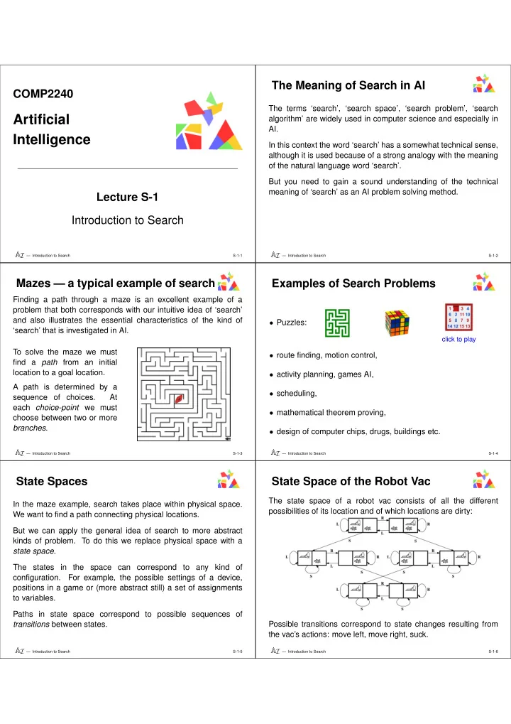
State Space of the Robot Vac

The state space of a robot vac consists of all the different possibilities of its location and of which locations are dirty: Possible transitions correspond to state changes resulting from the vac’s actions: move left, move right, suck. AI — Introduction to Search

S-1-6

SLIDE 2

Search Spaces

A search space is essentially just a state space, in which we have an initial state and one or more goal states. Given a search space, a solution to the search problem is a path consisting of a sequence of connected states, starting at the initial state and ending at one of the goal states. Consider the state space of the robot vac as a search space. What might be the goal state(s) ? Identify possible paths from the top left state to a goal state? Which paths are best? AI — Introduction to Search

S-1-7

Types of Search Problem

• Type 1)

Find a solution: Search for a state or configuration satisfying known conditions. E.g. in scheduling we search for a timetable satisfying given constraints on when events can occur — such as Lecture A cannot be at the same time as Lecture B.

• Type 2)

Find a way to reach a solution: Search for a sequence of steps (actions) that lead from an initial state to a desired goal state (either a specific state or any state satisfying given conditions). E.g. we want to find a sequence of moving, picking up and placing actions that a robot can execute to lay a table. AI — Introduction to Search

S-1-8

• Type 3)

Find the best way to reach a solution: Search for an optimal sequence of steps (actions) that lead from an initial state to a goal state. An optimal sequence is one that has the lowest ‘cost’ (i.e. takes the least time or resources). NOTE: the terminology of type 1-3 search problems is not in general use. I just introduced it to organise my description of the variety of search problems. AI — Introduction to Search

S-1-9

Reducing Type 1 to Type 2

Type 1 search may on first consideration seem simpler than type 2, since we are only interested in finding an actual solution, not in the details of how to get there. However, if one tries to find a solution without considering how it can be constructed, the only applicable method would be to try all possible configurations and check whether each is indeed a solution (e.g. check all possible schedules to see if they satisfy the given conditions). Type 1 problems are normally reduced to Type 2 by considering that a solution can be constructed by a series of steps. (E.g. a timetable is constructed in stages by a sequence of assignments

• f time slots to events.)

AI — Introduction to Search

S-1-10

Formulating Problems as Search Problems

A huge variety of problems can be cast into the form of search

• problems. In order to apply a search approach we need to analyse

the problem as follows:

• Conceptualise possible solutions and intermediate stages

towards solutions as states (and identify an initial state).

• Identify transitions that allow a state to be transformed into other

successor states.

• Devise an algorithm that will systematically search through

possible paths from the initial state in order to find a path that ends in a goal. AI — Introduction to Search

S-1-11

Search Trees

The state space associated with a problem can in general be an arbitrary graph. Each node is a state and each arc represents a possible transition between states. However, in devising a search algorithm we normally treat the search space as if it were a tree. The root node is the initial state. The children of each state/node S are all those states/nodes that are reachable S by a single transition. (Note that if the graph of the state space contains loops, the corresponding tree will be infinite.) AI — Introduction to Search

S-1-12

SLIDE 3

Explicit vs Generated Search Spaces

For certain problems, we may actually have a tree (or graph) structure stored as data — i.e. we have an explicit representation

• f the search space.

But in many cases the search space is not explicitly represented, rather a search tree is generated during the execution of the search algorithm. To generate such a tree one needs an algorithm or set of rules which, given any state, can return a list of all possible successor states. For example, if a robot is in a given state, we need a way to determine all the actions it could execute, and what state it would end up in after executing each of these. AI — Introduction to Search

S-1-13

Characterising Successor States

In order to implement a search algorithm, we need a way of determining the possible successors to any given state. There are several ways one might do this:

• Set up a data structure (tree or graph) that explicitly represents

the successor relation.

• Give a set of actions and specify in what kinds of state they can

be executed, and how they transform the state to a new state (e.g. the actions of a robot, with pre-conditions and effects).

• Specify a way of choosing a possible next state and also a set
• f conditions to determine whether that state is indeed possible.

(e.g. in constructing a timetable, pick the next lecture from a list, assign a time/room for it and then check that no clashes occur. AI — Introduction to Search

S-1-14

Useless Paths

How do we know whether we are on a path that will lead to a solution? In general we don’t. We may just have to keep going and see if we eventually get to a goal state. However, we may get to a dead end — a state which has no successors. Alternatively, we may come to a state that we have already been in — we are in a loop. Search algorithms are most efficient and easiest to implement if there are simple ways to test if we have reached a dead end or are in a loop. AI — Introduction to Search

S-1-15

The 8-Queens Problem

The 8-queens (more generally n-queens) problem is the problem

• f finding a placement of 8 (or n) queens on a chess board (or

n × n grid), such that no queen can take any other queen. See http://www.hbmeyer.de/backtrack/achtdamen/eight.htm How can one formulate the 8-queens problem as a search problem? AI — Introduction to Search

S-1-16

Search Algorithms

Considerable research in computer science and AI has addressed the question of what is a good algorithm for (quickly) finding a solution path in a search tree. This is a crucial problem since:

• lots of real problems can be formulated as search,
• search trees even for quite simple problems tend to get get

pretty massive. (If each state has 5 successors and the shortest solution path consists of 12 transitions, then the corresponding search tree contains at least 512 = 244, 140, 625 states.) Many different search algorithms have been developed. AI — Introduction to Search

S-1-17

Breadth-First Search

Breadth-first search is perhaps the most conceptually simple. We start at the root an explore the tree by working our way down level by level. Testing each path to see if we have reached a goal. The following diagram shows the order in which nodes are tested: AI — Introduction to Search

S-1-18

SLIDE 4

Depth-First Search

With depth first search we follow a single path down as deep as we can go until either we reach a goal or a dead end. In the latter case we ‘backtrack’ up the path until we reach a branch that has not yet been tried. We then search down this new branch: AI — Introduction to Search

S-1-19

Search for Optimal Solutions

For certain problems we do not only want a solution but want the best possible solution. In order to tell what is an optimal solution we need some kind of measure of how good a solution is. In some cases this measure is determined by the goal state itself. (e.g. the timetable with the fewest 9 o’clock lectures is the best). In cases where we are more interested in the path (Type 2 search), we typically want to find a path that is quickest, easiest

• r cheapest to carry out.

Typically we assign a cost to each transition, and the cost of a path is simply the sum of the costs of each transition in the path. AI — Introduction to Search

S-1-20

Optimal Path Example

You are on holiday in Romania and want to drive from Arad to Bucharest as quickly as possible (see Russell and Norvig): How can we search for the shortest path? AI — Introduction to Search

S-1-21

Further Work

You are strongly recommended to read Chapter 3 of Russell and

• Norvig. This presents search in a somewhat different way (relating

it much more to intelligent agents), but the essential ideas are the same. The Wikipedia article on ‘search algorithms’ is not particularly good, but the articles on particular types of search (depth-first etc.) seem to be pretty high quality. Find out more about the breadth and depth first search strategies. Is one of these better than the other? If so, why? We will look at these in more detail next lecture. AI — Introduction to Search

S-1-22

AI — Introduction to Search

S-1-23

AI — Introduction to Search

S-1-24

SLIDE 5

COMP2240

Artificial Intelligence

Lecture S-2 Search Strategies and Algorithms

AI — Search Strategies and Algorithms

S-2-1

Overview

In this lecture we shall look in more detail at the different ways in which search algorithms can be implemented. We shall see that there are several very different strategies for exploring a search space. The performance of a particular strategy/algorithm depends very much on the kind of problem being tackled. (In this lecture we are looking at uninformed search, where the algorithm does not make use of any means of estimating how close it is to a solution. Informed search will be covered in the next lecture.) AI — Search Strategies and Algorithms

S-2-2

Learning Goals

• You should understand the most important properties of:

– search spaces (branching factor, boundedness, looping, ...), – search algorithms (completeness, time/space complexity,

• ptimality, ...).
• You should acquire a basic understanding of the programming

techniques that are used in implementing search algorithms.

• You should gain a knowledge of the basic principles behind the

most commonly used search strategies.

• You should be able to consider a search problem and make

sensible comments about what kind of strategy/algorithm is likely to work best for that problem. AI — Search Strategies and Algorithms

S-2-3

Properties of Search Problems/Spaces

Different problems give rise to search spaces with particular characteristics, which may help or hinder search algorithms:

• Branching

factor: the number (or average number)

• f

successors of each node.

• The state space may be finite or infinite.
• Paths through the space may or may not have loops.
• Maximum path length may be bounded or unbounded (if the

state space is infinite or has loops). Different representations of the same problem may result in search spaces with different characteristics. AI — Search Strategies and Algorithms

S-2-4

Properties of Search Algorithms

• Completeness — Is the algorithm guaranteed to find a solution

if one exists (given sufficient computational resources)?

• Time Complexity — How much time does the algorithm require

in relation to the depth of the solution? (Usually proportional to the number of nodes that are generated.)

• Space Requirements — How much memory does the algorithm

require in relation to the depth of the solution? (Usually proportional to the number of nodes that need to be stored.)

• Optimality — Is the algorithm guaranteed to find the best

solution? (Given some measure on the cost of a solution.) AI — Search Strategies and Algorithms

S-2-5

Implementation Techniques

• Explicit representation of node set and implementation of

choice algorithm for node expansion.

• Recursive Algorithm. In the recursive algorithm approach the

nodes are not represented explicitly but are explicit in the execution sequence of the algorithm. (This approach is well-suited to depth-first search.) AI — Search Strategies and Algorithms

S-2-6

SLIDE 6

State Representation

The basis of nearly all search algorithms is a representation of the states that make up the search space. In Python, a state space for a robot moving items between rooms could be represented as follows:

initial_state = [ (’locked’, ’door_kl’), (’unlocked’, ’door_kg’), (’located’, ’robot’, ’kitchen’), (’located’, ’key’, ’garage’ ), (’located’, ’ring’, ’larder’ ) ]

In Prolog, a state in the famous missionaries and cannibals problem could be represented by: [boat, m, m, c, c] + [m, c] AI — Search Strategies and Algorithms

S-2-7

Nodes and Node Expansion

All standard search algorithms treat the search space as a tree. Each node in the tree corresponds to a state. Each node (except the root) has a parent and 0 or more children. The children are the nodes that are reachable by one action. Node expansion is the process of computing the children of a given node. This is often done in two stages: 1) Determine what actions are possible, 2) Determine the successor state that results from each of these actions. AI — Search Strategies and Algorithms

S-2-8

The Fringe

The fringe is the set of nodes that have been generated by the search procedure, but have not been expanded. The search strategy can be characterised as the method by which an algorithm chooses which of the fringe nodes to expand. When a node is expanded it is no longer part of the fringe. But its children are then added to the fringe. AI — Search Strategies and Algorithms

S-2-9

Node Queueing

One way to control the way in which fringe nodes are chosen for expansion is to organise the fringe nodes as a queue — i.e. a list

• f nodes from which we draw from one end.

Search using a queueing system proceeds according to the following repeated sequence:

• Take first node from the queue
• If the node satisfies the goal, return the node.

(search successful)

• Otherwise, expand the node to find its children.
• Add the children to the queue.

If the queue becomes empty the search fails. AI — Search Strategies and Algorithms

S-2-10

Most Widely Used Strategies

• Depth First

Modifications of depth first include: – Depth Limited – Iterative Deepening Often used with loop checking and/or random branch choice. (Choice according to cost often not useful.)

• Breadth First

Modifications of depth first include: – Uniform Cost (not exactly breadth-first) – Bi-Directional Search Can be combined with removal of duplicate states and other node pruning techniques. AI — Search Strategies and Algorithms

S-2-11

Depth-First Tree Expansion

AI — Search Strategies and Algorithms

S-2-12

SLIDE 7

Depth-First Search for 8-Puzzle

AI — Search Strategies and Algorithms

S-2-13

Properties of Depth-First Search

• Relatively modest memory requirements (∝ path length to

solution). We only need to store nodes in a single active branch.

• Not usually optimal — often explores branches that are much

longer that the shortest to a solution.

• Not complete unless all paths terminate.
• Loop checking is often required to eliminate useless infinitely

repeating branches.

• Can be implemented by a LIFO Node-Queueing System — i.e.

add generated child nodes to the front of the queue. AI — Search Strategies and Algorithms

S-2-14

Breadth-First Tree Expansion

In the breadth-first strategy we always expand nodes that are nearest (or equal nearest) to the root of the search tree. Large memory requirement, since the number of nodes in the fringe is of the order of

bd

where b is the (average) branching factor, and d is the depth of the tree. AI — Search Strategies and Algorithms

S-2-15

Properties of Breadth-First Search

• Complete as long as branching factor is finite
• Finds
• ptimal

path first, provided that path cost is a monotonically increasing function of depth

• Execution time increases exponentially as the minimum path

length to solution increases.

• Memory requirements can be very large.

Need to store the whole tree down to the level of the solution, so memory exponential function of minimum path length to solution.

• Can be implemented by a FIFO Node-Queueing System — i.e.

add generated child nodes to the end of the queue. AI — Search Strategies and Algorithms

S-2-16

Depth-Limited Search

A major problem with depth-first search is that it is incomplete unless every branch is eventually terminated either by: reaching a goal or dead end, looping to a state that occurs earlier in the branch (we need to test for this). If there are non-terminating branches, the search may run forever without either reaching a goal state or determining that the problem is insoluble. In a depth-limited search we set a maximum length of path that will be searched. Depth-limited search is still usually incomplete (unless there is some reason why there must be a solution with a path within the limit). However, at least the search algorithm is guaranteed to terminate. AI — Search Strategies and Algorithms

S-2-17

Iterative Deepening

The iterative deepening strategy consists of repeated use of depth-limited depth first search, where the depth limit is increased (by one or more) each time until a solution is found. Combines benefits of breath and depth first search:

• Modest memory requirements (same as depth first)
• Complete when branching factor is finite
• Optimal when path cost is non-decreasing function of depth

The downside is that execution time is likely to be large. AI — Search Strategies and Algorithms

S-2-18

SLIDE 8

Iterative Deepening in Action

AI — Search Strategies and Algorithms

S-2-19

Uniform Cost Search

Uniform Cost search is a varient of breadth-first search. In standard breadth-first search, we are always expanding nodes that are closest to the initial state in terms of the number of actions in their path. But in Uniform Cost search we expand the nodes that are closest to the initial state in terms of the cost of their path. Consequently, nodes on the fringe will have approximately equal costs. If the cost of all actions is the same, Uniform Cost search is equivalent to standard breadth first-search. Uniform Cost search can be implemented by a queue that is

• rdered by means of the path cost function (lowest cost first).

AI — Search Strategies and Algorithms

S-2-20

Direction of Search

Until now, we have been thinking of search as progressing from an initial state towards a goal state. However, it is sometimes better to search backwards. In other words we start from the goal and then look for states that can reach the goal by one action. We then proceed to look at states that can reach these states by

• ne action, and continue until (hopefully) we reach the initial state.

This is useful when the backwards branching factor is lower than the forwards branching factor. Backwards search is difficult to implement if there are many goal states, or if the state transitions are difficult to define in the reverse direction. AI — Search Strategies and Algorithms

S-2-21

Bi-Directional Search

Bi-Directional Search is a strategy where the search space is explored from both the initial state and the goal state. A solution is found when the forward and backwards search paths meet at some state. Questions: What is the advantage of this? What search strategies would it be sensible to employ as the forward and backward components of a bi-directional search? AI — Search Strategies and Algorithms

S-2-22

Conclusion

• Different search problems give rise to search spaces with

different structural characteristics.

• A range of different search strategies have been devised, which

vary in terms of their computational properties.

• Certain general programming techniques can be applied to

many different search problems and strategies.

• The effective use of search techniques requires constructing

an appropriate search-space representation and matching the search strategy to the characteristics of this space. AI — Search Strategies and Algorithms

S-2-23

Further Work

Python Code Examples: Example search algorithm implmentations will be posted on the VLE. Reading Suggesion: Simon Colton of Imperial College London, has a nice set of notes

• n AI.

For a very good account of search techniques have a look at his lecture notes on Search in Problem Solving at:

http://www.doc.ic.ac.uk/~sgc/teaching/pre2012/v231/lecture3.html

Some other parts of Simon’s course may be useful. The whole course material is at:

http://www.doc.ic.ac.uk/~sgc/teaching/pre2012/v231/

AI — Search Strategies and Algorithms

S-2-24

SLIDE 9

COMP2240

Artificial Intelligence

Lecture S-3 Informed (Heuristic) Search

AI — Informed (Heuristic) Search

S-3-1

Overview

This lecture covers the following topics:

• The meaning of a heuristic and its use in search algorithms.
• Examples of heuristics that are useful for particular search

problems.

• Informed Search Methods

– Greedy Best First search – A* Search This material is covered in Russell and Norvig Chapter 4. AI — Informed (Heuristic) Search

S-3-2

Heuristics

A heuristic is a rule of thumb — a good way of evaluating something, which is not theoretically perfect. In the context of search heuristic functions are used to compute estimates to guide the choice of nodes to expand. Typically we use a heuristic function that estimates the cost of getting from any given state to a goal state — i.e. the cost of the remaining path to a goal. Thus we want a function that gives a low value for states that we think are likely to be near to the solution and a high value for those that are far from the solution. AI — Informed (Heuristic) Search

S-3-3

What Makes a Good Heuristic?

What makes a good heuristic depends on the problem under consideration. Finding a good heuristic often requires some ingenuity. In the case of a route-planning search, a simple and often very effective heuristic is given by estimating the cost from each node to the goal to be the straight line distance from the node to the goal. Clearly the straight line distance will always be less than or equal to the distance along an actual path of the network. This heuristic is usually good because for many transport networks, when choosing the next leg of the route, it is mostly best to head towards the destination (though there can be exceptions!). AI — Informed (Heuristic) Search

S-3-4

A Problematic Case

Exercise: draw an example of a network, where using the least straight line distance heuristic will not be a good guide to finding the shortest route from A to B (indicate these nodes): AI — Informed (Heuristic) Search

S-3-5

Search Using Heuristics

The use of heuristics gives us a new way to guide a search algorithm that was not available with uninformed search. A heuristic function gives an indication of which nodes are likely to be the ‘best’ choices in the search for a solution. In queue-based search, the heuristic can be used to order the nodes in the queue. This is called best-first search. Of course, since a heuristic only gives an estimate of how close a node is likely to be to the solution, it will not always tell us which is actually the best. If we had a perfect measure we would not need a search algorithm at all. We could directly compute a path straight to the solution. AI — Informed (Heuristic) Search

S-3-6

SLIDE 10

Greedy Search

The simplest ‘best-first’ search algorithm simply orders the node queue according to the heuristic function. We always expand the node with the lowest value of the heuristic. The children of the expanded node are then merged into the queue according to the heuristic function ordering. AI — Informed (Heuristic) Search

S-3-7

Greedy Search Example

AI — Informed (Heuristic) Search

S-3-8

Properties of Greedy Search

Greedy search is simple and can be effective for certain kinds of search problem. However, it has some severe limitations:

• Susceptible to ‘false starts’ and other inefficient behaviour.
• Incomplete — if there are infinite branches it may carry on

forever, never trying alternatives that were rated less good by the heuristic but lead to a solution.

• Non-Optimal — no guarantee of finding lowest cost solution.
• Time and Space Complexity are both bn, were b is branching

factor and n is maximum depth of the search tree. AI — Informed (Heuristic) Search

S-3-9

A* (A-Star) Search

The clever but still relatively simply A* algorithm avoids many problems of greedy search. It does this by also taking account the cost expended in getting to a node (like the Uniform Cost algorithm). In A* search we expand nodes in order of the lowest value of the heuristic f(n): f(n) = c(n) + h(n) where c(n) is the cost of getting from the initial state to node n, and h(n) is a heuristic estimate of the cost of getting from node n to a goal state. Thus, f(n) gives an estimate of the total cost of getting from initial state to a goal going via node n. AI — Informed (Heuristic) Search

S-3-10

A* Example

AI — Informed (Heuristic) Search

S-3-11

Admissible Heuristics

For reasons that will soon become apparent, A* search is usually conducted using a heuristic function that is admissible, in the following sense: A heuristic h is admissible iff its estimate h(n) of the cost to get from node n to a goal state is always less than or equal to the actual cost of the minimum path from n to a goal state. Admissible heuristics are often described as optimistic, since they tend to indicate that the goal is closer than it actually is. Question: Is the straight-line distance heuristic admissible for route search problems? AI — Informed (Heuristic) Search

S-3-12

SLIDE 11

Properties of A* Search

Provided it is used with an admissible heuristic, A* search has some pretty nice properties:

• Complete — it always finds a solution if there is one.
• Optimal — it will always find a minimum cost path to a solution.
• Time and Space Complexity — both exponential in solution path

length. :-( Admissibility is required for these properties as it ensures that no node is ignored because it is considered further from the solution that it actually is. (See Russell and Norvig Chapter 4 for further explanation and proofs.) AI — Informed (Heuristic) Search

S-3-13

Path Finding Demo

The following web page has a nice visual demo of path finding using search techniques. It enables you to choose from several

• f the most common search strategies and heuristics suitable for

finding paths (on a grid) in the presence of obstacles. http://qiao.github.io/PathFinding.js/visual/ AI — Informed (Heuristic) Search

S-3-14

Heuristic Finding Exercise

Try to think of potentially usefull heuristic functions for the following kinds of search problem:

• The 8 or 15 sliding tile puzzles.
• A robot that has to collect items from different locations and

deposit them in some target location.

• The ‘Knight’s Tour’ puzzle. (tricky)

AI — Informed (Heuristic) Search

S-3-15

Conclusion

This lecture has introduced the idea of informed search guided by a heuristic function that estimates the distance/cost of any given node to a goal. We have considered what kinds of heuristic might be useful for particular search problems. We have examined (and hopefully understood) the workings of two heuristic search algorithms:

• the simple greedy ‘best-first’ search (which doesn’t always

make the best choices),

• and the clever A*, which has nice properties but can still take

loads of time and memory. AI — Informed (Heuristic) Search

S-3-16

AI — Informed (Heuristic) Search

S-3-17

AI — Informed (Heuristic) Search

S-3-18

SLIDE 12

COMP2240

Artificial Intelligence

Lecture S-4 More Heuristic Search

AI — More Heuristic Search

S-4-1

Overview

This lecture covers the following topics:

• Choice and comparison of heuristics.
• Iterative Improvement strategies.

– Hill Climbing AI — More Heuristic Search

S-4-2

The 8-Puzzle Example

This example will illustrate the choice between different heuristics. The 8-Puzzle involves sliding tiles on a 3x3 grid, where one space is empty. A move consists of sliding one of the tiles into the empty

• space. The idea is to get from an arbitrary starting configuration

to some chosen goal state:

Initial State 2 4 8 5 1 7 3 6 right = ⇒ 2 4 8 5 1 7 3 6 up = ⇒ 2 4 8 5 3 1 7 6 = ⇒ ... ... = ⇒ 2 3 1 8 4 7 6 5 up = ⇒ 1 2 3 8 4 7 6 5 left = ⇒ Goal State 1 2 3 8 4 7 6 5

AI — More Heuristic Search

S-4-3

Choice of Heuristic

There are two relatively straightforward heuristics that one might apply to the 9-Puzzle:

• 1. h(state) = the numer of tiles in state that are not in the place

they should be in the goal state.

• 2. h(state) = the sum of Manhattan Distances from the position of

each tiles in state to its position in the goal state. (The Manhattan Distance is the sum of distances in the horizontal and vertical directions.) Which of this are admissible heuristics? Which heuristic is the best? AI — More Heuristic Search

S-4-4

Evaluating Heuristics

One way to evaluate heuristics is by calculating their Effective Branching Factor over a set of problems by comparison with breadth first search. In breadth-first search the number of nodes N generated in exploring a search tree with branching factor b to a depth d is given by: N = 1 + b + b2 + . . . + bd If we use some heuristic function, this equation is not applicable, but we will still have values for N and d for each successful search. From these we use the above formula to calculate b to calculate the effective branching factor b, as if we were using ordinary breadth first search. By averaging over a number of problems we get a good measure of the heuristic (closest to 1 is best). AI — More Heuristic Search

S-4-5

Comparison of Admissible Heuristics

Recall that a heuristic is admissible if and only if it always underes- timates the distance to a goal. If h1 and h2 are two heuristics for the same problem and for all states s we always have h2 ≥ h1 we shat that h2 dominates h1. For admissible heuristics the dominant heuristic is always better. Why? Since the heuristics do not overestimate the distance to the goal, a higher value is always closer to the true distance — hence it is more accurate. More accurate heuristics give better guidance towards the goal. AI — More Heuristic Search

S-4-6

SLIDE 13

Finding Heuristics by Constraint Relaxation

A good way of finding a heuristic is by considering a distance measure for a simpler, less constrained version of the problem. For example the 8-Puzzle can be considered as the problem of moving tiles from one grid configuration to another under the following conditions:

• nly one tile can move at a time,
• a tile can only move one space at a time,
• a tile cannot move on top of another tile.

Consider how by relaxing (i.e. removing) one or more of these constraints we get problems where the distance to the goal is exactly given by one of the 8-Puzzle heuristics mentioned above (number of missplaced tiles and total Manhattan distance). AI — More Heuristic Search

S-4-7

Iterative Improvement Algorithms

In the algorithms we have looked at so far, a solution has been cast as a sequence of steps to a goal. In cases where only the goal is important (Type 1) we have considered steps that build towards a complete solution in stages. An alternative approach to Type 1 problems is Iterative Improvement, whose basic idea is: Start with a complete (but defective or sub-optimal) state configuration and make modifications to improve its quality. When doing iterative improvement we normally use a heuristic that is a positive measure of ‘goodness’ of each state (high is good). Hence, we look for modifications that increase the value of the heuristic. AI — More Heuristic Search

S-4-8

Surface of Heuristic Function

We can visualise the heuristic function as a surface: AI — More Heuristic Search

S-4-9

Hill Climbing

• Moves in direction of increasing value (uphill)
• Terminates at a peak
• Shoulders and Plateaux are problems
• Many variants:

– Stochastic hill climbing ∗ Selects uphill moves at random ∗ Probability based on steepness – Random-restart hill climbing

• Hill Climbing never goes downhill and will therefore get stuck on

a local maximum AI — More Heuristic Search

S-4-10

Iterative Improvement for Constraint Satisfaction

Iterative Improvement can also be used for constraint satisfaction type problems. In such cases we allow states to violate certain constraints and then define a heuristic that measures how good a state in terms

• f the number of constraints that are violated.

For instance in the N-Queens problem we can use a heuristic based on the number of ‘clashes’ arising in a state — ie the number of queens that lie on a taking move of another queen. Iterative improvement would then proceed by looking for ways to move one of the queens that reduces the number of clashes. AI — More Heuristic Search

S-4-11

Conclusion

• We have looked in more detail at the nature of heuristics and

how they can be identified and compared.

• We also considered Iterative Improvement techniques such

as the Hill Climbing search strategy, where we try to make successive improvements on an initial state. AI — More Heuristic Search

S-4-12

SLIDE 14

COMP2240

Artificial Intelligence

Lecture S-5 Uniform Cost Search Example

AI — Uniform Cost Search Example

S-5-1

Overview

When carrying out uniform cost search we always expand the node that has the least total cost to reach from the goal. The total cost to reach a node is obtained by adding the cost of each action along the path from the start node to that node. If several nodes have the same total cost we can pick several of them. (Note: if all actions have the same cost, then uniform cost search is the same as breadth first search.) AI — Uniform Cost Search Example

S-5-2

Uniform Cost Search 1

S AI — Uniform Cost Search Example

S-5-3

Uniform Cost Search 2

S A

13

B

5

S AI — Uniform Cost Search Example

S-5-4

Uniform Cost Search 3

S A

13

B

5

E

7

F

20

G

8

H

17

S, B AI — Uniform Cost Search Example

S-5-5

Uniform Cost Search 4

S A

13

B

5

E

7

F

20

G

8

H

17

J

12

S, B, E AI — Uniform Cost Search Example

S-5-6

SLIDE 15

Uniform Cost Search 5

S A

13

B

5

E

7

F

20

G

8

H

17

J

12

K

11

S, B, E, G AI — Uniform Cost Search Example

S-5-7

Uniform Cost Search 6

S A

13

B

5

E

7

F

20

G

8

H

17

J

12

K

11

Goal C

16

S, B, E, G, K AI — Uniform Cost Search Example

S-5-8

Uniform Cost Search 7

S A

13

B

5

E

7

F

20

G

8

H

17

J

12

K

11

Goal c

16

Goal B

15

S, B, E, G, K, J AI — Uniform Cost Search Example

S-5-9

Uniform Cost Search 8

S A

13

B

5

E

7

F

20

G

8

H

17

J

12

K

11

Goal c

16

Goal b

15

C

19

D

21

S, B, E, G, K, J, A AI — Uniform Cost Search Example

S-5-10

Uniform Cost Search 9

Optimum Path: S, B, E, J, Goal b S A

13

B

5

E

7

F

20

G

8

H

17

J

12

K

11

Goal c

16

Goal b

15

C

19

D

21

S, B, E, G, K, J, A, Goal b AI — Uniform Cost Search Example

S-5-11