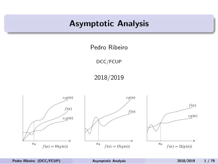
Asymptotic Analysis Pedro Ribeiro DCC/FCUP 2018/2019 Pedro - - PowerPoint PPT Presentation

Asymptotic Analysis

Pedro Ribeiro

DCC/FCUP

2018/2019

Pedro Ribeiro (DCC/FCUP) Asymptotic Analysis 2018/2019 1 / 79

Motivational Example - TSP

Traveling Salesman Problem (Euclidean TSP version) Input: a set S of n points in the plane Output: the smallest possible path that starts on a point, visits all other points of S and then returns to the starting point. An example:

Pedro Ribeiro (DCC/FCUP) Asymptotic Analysis 2018/2019 2 / 79

Motivational Example - TSP

A possible (greedy) algorithm - nearest neighbour p1 ← random point i ← 1 While (there are still points to visit) do i ← i + 1 pi ← nearest non visited neighbour of point pi−1 return path p1 → p2 → . . . → pn → p1

Pedro Ribeiro (DCC/FCUP) Asymptotic Analysis 2018/2019 3 / 79

Motivational Example - TSP

Seems to work... ⇒

Pedro Ribeiro (DCC/FCUP) Asymptotic Analysis 2018/2019 4 / 79

Motivational Example - TSP

But it is does not work for all instances! (Note: starting with the leftmost point would not solve the problem)

Pedro Ribeiro (DCC/FCUP) Asymptotic Analysis 2018/2019 5 / 79

Motivacional Example - TSP

Another possible (greedy) algorithm For i ← 1 to (n − 1) do Add connection between closest pair of points such that they are in different connected components Add connection between the two ”extremes” of the created path return the cyclic path created

Pedro Ribeiro (DCC/FCUP) Asymptotic Analysis 2018/2019 6 / 79

Motivational Example - TSP

It does not work for all cases!

Pedro Ribeiro (DCC/FCUP) Asymptotic Analysis 2018/2019 7 / 79

Motivational Example - TSP

How to solve the problem then? A possible algorithm (exhaustive search a.k.a. ”brute force”) Pmin ← any permutation of the points in S For Pi ← each of the permutations of points in S If (cost(Pi) < cost(Pmin)) then Pmin ← Pi retorn Path formed by Pmin A correct algorithm, but extremely slow! P(n) = n! = n × (n − 1) × . . . × 1 For instance, P(20) = 2, 432, 902, 008, 176, 640, 000 For a set of 20 points, even the fastest computer in the world would not solve it! (how long would it take?)

Pedro Ribeiro (DCC/FCUP) Asymptotic Analysis 2018/2019 8 / 79

Motivational Example - TSP

The present problem is a restricted version (euclidean) of one of the most well known ”classic” hard problems, the Travelling Salesman Problem (TSP) This problem has many possible applications Ex: genomic analysis, industrial production, vehicle routing, ... There is no known efficient solution for this problem (with optimal results, not just approximated) The presented solution has O(n!) complexity The Held-Karp algorithm has O(2nn2) complexity (this notation will be the focus of this class) TSP belongs to the class of NP-hard problems The decision version belongs to the class of NP-complete problems (we will also talk about this at the end of the semester)

Pedro Ribeiro (DCC/FCUP) Asymptotic Analysis 2018/2019 9 / 79

An experience - how many instructions

How many instructions per second on a current computer? (just an approximation, an order of magnitude) On my notebook, about 109 instructions At this velocity, how much time for the following quantities of instructions? Quant. 100 1000 10000 N < 0.01s < 0.01s < 0.01s N2 < 0.01s < 0.01s 0.1s N3 < 0.01s 1.00s 16 min N4 0.1s 16 min 115 days 2N 1013 years 10284 years 102993 years n! 10141 years 102551 years 1035642 years

Pedro Ribeiro (DCC/FCUP) Asymptotic Analysis 2018/2019 10 / 79

An experience: - Permutations

Let’s go back to the idea of permutations Exemple: the 6 permutations of {1, 2, 3} 1 2 3 1 3 2 2 1 3 2 3 1 3 1 2 3 2 1 Recall that the number of permutations can be computed as: P(n) = n! = n × (n − 1) × . . . × 1 (do you understand the intuition on the formula?)

Pedro Ribeiro (DCC/FCUP) Asymptotic Analysis 2018/2019 11 / 79

An experience: - Permutations

What is the execution time of a program that goes through all permutations? (the following times are approximated, on my notebook) (what I want to show is order of growth) n ≤ 7: < 0.001s n = 8: 0.001s n = 9: 0.016s n = 10: 0.185s n = 11: 2.204s n = 12: 28.460s . . . n = 20: 5000 years ! How many permutations per second? About 107

Pedro Ribeiro (DCC/FCUP) Asymptotic Analysis 2018/2019 12 / 79

On computer speed

Will a faster computer be of any help? No! If n = 20 → 5000 years, hypothetically:

◮ 10x faster would still take 500 years ◮ 5,000x would still take 1 year ◮ 1,000,000x faster would still take two days, but

n = 21 would take more than a month n = 22 would take more than a year!

The growth rate of the execution time is what matters! Algorithmic performance vs Computer speed A better algorithm on a slower computer will always win against a worst algorithm on a faster computer, for sufficiently large instances

Pedro Ribeiro (DCC/FCUP) Asymptotic Analysis 2018/2019 13 / 79

Why worry?

What can we do with execution time/memory analysis? Prediction How much time/space does an algorithm need to solve a problem? How does it scale? Can we provide guarantees on its running time/memory? Comparison Is an algorithm A better than an algorithm B? Fundamentally, what is the best we can possibly do on a certain problem? We will study a methodology to answer these questions We will focus mainly on execution time analysis

Pedro Ribeiro (DCC/FCUP) Asymptotic Analysis 2018/2019 14 / 79

Random Access Machine (RAM)

We need a model that is generic and independent from the language and the machine. We will consider a Random Access Machine (RAM)

◮ Each simple operation (ex: +, −, ←, If) takes 1 step ◮ Loops and procedures, for example, are not simple instructions! ◮ Each access to memory takes also 1 step

We can measure execution time by... counting the number of steps as a function of the input size n: T(n). Operations are simplified, but this is useful Ex: summing two integers does not cost the same as dividing two reals, but we will see that on a global vision, these specific values are not important

Pedro Ribeiro (DCC/FCUP) Asymptotic Analysis 2018/2019 15 / 79

Random Access Machine (RAM)

A counting example

A simple program int count = 0; for (int i=0; i<n; i++) if (v[i] == 0) count++ Let’s count the number of simple operations: Variable declarations 2 Assignments: 2 ”Less than” comparisons n + 1 ”Equality” comparisons: n Array access n Increment between n and 2n

Pedro Ribeiro (DCC/FCUP) Asymptotic Analysis 2018/2019 16 / 79

Random Access Machine (RAM)

A counting example

A simple program int count = 0; for (int i=0; i<n; i++) if (v[i] == 0) count++ Total number of steps on the worst case: T(n) = 2 + 2 + (n + 1) + n + n + 2n = 5 + 5n Total number of steps on the best case: T(n) = 2 + 2 + (n + 1) + n + n + n = 5 + 4n

Pedro Ribeiro (DCC/FCUP) Asymptotic Analysis 2018/2019 17 / 79

Types of algorithm analysis

Worst Case analysis: (the most common) T(n) = maximum amount of time for any input of size n Average Case analysis: (sometimes) T(n) = average time on all inputs of size n Implies knowing the statistical distribution of the inputs Best Case analysis: (”deceiving”) It’s almost like ”cheating” with an algorithm that is fast just for some of the inputs

Pedro Ribeiro (DCC/FCUP) Asymptotic Analysis 2018/2019 18 / 79

Types of algorithm analysis

Pedro Ribeiro (DCC/FCUP) Asymptotic Analysis 2018/2019 19 / 79

Asymptotic Notation

We need a mathematical tool to compare functions On algorithm analysis we use Asymptotic Analysis: ”Mathematically”: studying the behaviour of limits (as n → ∞) Computer Science: studying the behaviour for arbitrary large input

• r

”describing” growth rate A very specific notation is used: O, Ω, Θ, o, ω It allows to focus on orders of growth

Pedro Ribeiro (DCC/FCUP) Asymptotic Analysis 2018/2019 20 / 79

Asymptotic Notation

Definitions

f(n) = O(g(n))

It means that c × g(n) is an upper bound of f (n)

f(n) = Ω(g(n))

It means that c × g(n) is a lower bound of f (n)

f(n) = Θ(g(n))

It means that c1 × g(n) is a lower bound of f (n) and c2 × g(n) is an upper bound of f (n) Note: ∈ could be used instead of =

Pedro Ribeiro (DCC/FCUP) Asymptotic Analysis 2018/2019 21 / 79

Asymptotic Notation

A graphical depiction

Θ O Ω

The definitions imply an n from which the function is bounded. The small values of n do not ”matter”.

Pedro Ribeiro (DCC/FCUP) Asymptotic Analysis 2018/2019 22 / 79

Asymptotic Notation

Formalization

f(n) = O(g(n)) if there exist positive constants n0 and c such that f (n) ≤ c × g(n) for all n ≥ n0 f(n) = Ω(g(n)) if there exist positive constants n0 and c such that f (n) ≥ c × g(n) for all n ≥ n0 f(n) = Θ(g(n)) if there exist positive constants n0, c1 and c2 such that c1 × g(n) ≤ f (n) ≤ c2 × g(n) for all n ≥ n0 f(n) = o(g(n)) if for any positive constant c there exists n0 such that f (n) < c × g(n) for all n ≥ n0 f(n) = ω(g(n)) if for any positive constant c there exists n0 such that f (n) > c × g(n) for all n ≥ n0

Pedro Ribeiro (DCC/FCUP) Asymptotic Analysis 2018/2019 23 / 79

Asymptotic Notation

Analogy

Comparison between two functions f and g and two numbers a and b: f (n) = O(g(n)) is like a ≤ b upper bound at least as good as f (n) = Ω(g(n)) is like a ≥ b lower bound at least as bad as f (n) = Θ(g(n)) is like a = b tight bound as good as f (n) = o(g(n)) is like a < b strict upper b. strictly better than f (n) = ω(g(n)) is like a > b strict lower b. strictly worst than

Pedro Ribeiro (DCC/FCUP) Asymptotic Analysis 2018/2019 24 / 79

Asymptotic Notation

A few consequences

f (n) = Θ(g(n)) → f (n) = O(g(n)) and f (n) = Ω(g(n)) f (n) = O(g(n)) → f (n) = ω(g(n)) f (n) = Ω(g(n)) → f (n) = o(g(n)) f (n) = o(g(n)) → f (n) = Ω(g(n)) f (n) = ω(g(n)) → f (n) = O(g(n)) f (n) = Θ(g(n)) → g(n) = Θ(f (n)) f (n) = O(g(n)) → g(n) = Ω(f (n)) f (n) = Ω(g(n)) → g(n) = O(f (n)) f (n) = o(g(n)) → g(n) = ω(f (n)) f (n) = ω(g(n)) → g(n) = o(f (n))

Pedro Ribeiro (DCC/FCUP) Asymptotic Analysis 2018/2019 25 / 79

Asymptotic Notation

A few practical rules

Multiplying by a constant does not affect: Θ(c × f (n)) = Θ(f (n)) 99 × n2 = Θ(n2) On a polynomial of the form axnx + ax−1nx−1 + . . . + a2n2 + a1n + a0 we can focus on the term with the largest exponent: 3n3 − 5n2 + 100 = Θ(n3) 6n4 − 202 = Θ(n4) 0.8n + 224 = Θ(n) More than that, on a sum we can focus on the dominant term: 2n + 6n3 = Θ(2n) n! − 3n2 = Θ(n!) n log n + 3n2 = Θ(n2)

Pedro Ribeiro (DCC/FCUP) Asymptotic Analysis 2018/2019 26 / 79

Asymptotic Notation

Dominance

When is a function better than another? If we want to minimize time, ”smaller” functions are better A function dominates another if as n grows it keeps getting larger Mathematically: f (n) ≫ g(n) if limn→∞ g(n)/f (n) = 0 Dominance Relations

n! ≫ 2n ≫ n3 ≫ n2 ≫ n log n ≫ n ≫ log n ≫ 1

Pedro Ribeiro (DCC/FCUP) Asymptotic Analysis 2018/2019 27 / 79

Asymptotic Growth

A practical view

If an operation takes 10−9 seconds...

log n n n log n n2 n3 2n n! 10

< 0.01s < 0.01s < 0.01s < 0.01s < 0.01s < 0.01s < 0.01s

20

< 0.01s < 0.01s < 0.01s < 0.01s < 0.01s < 0.01s

77 years 30

< 0.01s < 0.01s < 0.01s < 0.01s < 0.01s

1.07s 40

< 0.01s < 0.01s < 0.01s < 0.01s < 0.01s

18.3 min 50

< 0.01s < 0.01s < 0.01s < 0.01s < 0.01s

13 days 100

< 0.01s < 0.01s < 0.01s < 0.01s < 0.01s

1013years 103

< 0.01s < 0.01s < 0.01s < 0.01s

1s 104

< 0.01s < 0.01s < 0.01s

0.1s 16.7 min 105

< 0.01s < 0.01s < 0.01s

10s 11 days 106

< 0.01s < 0.01s

0.02s 16.7 min 31 years 107

< 0.01s

0.01s 0.23s 1.16 days 108

< 0.01s

0.1s 2.66s 115 days 109

< 0.01s

1s 29.9s 31 years

Pedro Ribeiro (DCC/FCUP) Asymptotic Analysis 2018/2019 28 / 79

Asymptotic Notation

Common Functions

Function Name Examples 1 constant summing two numbers log n logarithmic binary search, inserting in a heap n linear 1 loop to find maximum value n log n linearithmic sorting (ex: mergesort, heapsort) n2 quadratic 2 loops (ex: verifying, bubblesort) n3 cubic 3 loops (ex: Floyd-Warshall) 2n exponential exhaustive search (ex: subsets) n! factorial all permutations

Pedro Ribeiro (DCC/FCUP) Asymptotic Analysis 2018/2019 29 / 79

Asymptotic Growth

Drawing functions

An useful program for drawing functions is gnuplot. (comparing 2n3 with 100n2 for 1 ≤ n ≤ 100) gnuplot> plot [1:70] 2*x**3, 100*x**2 gnuplot> set logscale xy 10 gnuplot> plot [1:10000] 2*x**3, 100*x**2 (which grows faster: √n or log2 n?) gnuplot> plot [1:1000000] sqrt(x), log(x)/log(2)

Pedro Ribeiro (DCC/FCUP) Asymptotic Analysis 2018/2019 30 / 79

Asymptotic Analysis

A few more examples

A program has two pieces of code A and B, executed one after the

• ther, with A running in Θ(n log n) and B in Θ(n2).

The program runs in Θ(n2), because n2 ≫ n log n A program calls n times a function Θ(log n), and then it calls again n times another function Θ(log n) The program runs in Θ(n log n) A program has 5 loops, all called sequentially, each one of them running in Θ(n) The program runs in Θ(n) A program P1 has execution time proportional to 100 × n log n. Another program P2 runs in 2 × n2. Which one is more efficient? P1 is more efficient because n2 ≫ n log n. However, for a small n, P2 is quicker and it might make sense to have a program that calls P1 or P2 depending on n.

Pedro Ribeiro (DCC/FCUP) Asymptotic Analysis 2018/2019 31 / 79

Analyzing the complexity of programs

Let’s see more concrete examples: Case 1 Loops (and summations) Case 2 Recursive Functions (and recurrences)

Pedro Ribeiro (DCC/FCUP) Asymptotic Analysis 2018/2019 32 / 79

Loops and Summations

A typical loop count ← For i ← 1 to 1000 For j ← i to 1000 count ← count + 1 write(count) What does this program write? 1000 + 999 + 998 + 997 + . . . .. + 2 + 1

Pedro Ribeiro (DCC/FCUP) Asymptotic Analysis 2018/2019 33 / 79

Loops and Summations

Arithmetic progression: a sequence of numbers such that the difference d between the consecutive terms is constant. We will call a1 to the first term. 1, 2, 3, 4, 5, . . . ... (d = 1, a1 = 1) 3, 5, 7, 9, 11, . . . ... (d = 2, a1 = 3) How to calculate the summation of an arithmetic progression? 1 + 2 + 3 + 4 + 5 + 6 + 7 + 8 = (1 + 8) + (2 + 7) + (3 + 6) + (4 + 5) = 4 × 9 Summation from ap to aq S(p, q) =

q

• i=p

ai = (q−p+1)×(ap+aq)

2

Summation of the first n terms Sn =

n

• i=1

ai = n×(a1+an)

2

Pedro Ribeiro (DCC/FCUP) Asymptotic Analysis 2018/2019 34 / 79

Loops and Summations

A typical loop count ← For i ← 1 to 1000 For j ← i to 1000 count ← count + 1 write(count) What does this program write? 1000 + 999 + 998 + 997 + . . . .. + 2 + 1 It writes S1000 = 1000×(1000+1)

2

= 500500

Pedro Ribeiro (DCC/FCUP) Asymptotic Analysis 2018/2019 35 / 79

Loops and Summations

A typical loop count ← For i ← 1 to n For j ← i to n count ← count + 1 write(count) What is the execution time? It is going to execute Sn increments: Sn =

n

• i=1

ai = n×(1+n)

2

= n+n2

2

= 1

2n2 + 1 2n.

It executes Θ(n2) steps

Pedro Ribeiro (DCC/FCUP) Asymptotic Analysis 2018/2019 36 / 79

Loops and Summations

If you want to know more about interesting summations on the context of CS, take a look at Appendix A of the Introduction to Algorithms book. Note that c loops do not imply Θ(nc)! A loop For i ← 1 to n For j ← 1 to 5 Θ(n) Another loop For i ← 1 to n For j ← 1 to i × i Θ(n3) (12 + 22 + 32 + . . . + n2 =

n

• i=1

i2 = n(n+1)(2n+1)

6

Pedro Ribeiro (DCC/FCUP) Asymptotic Analysis 2018/2019 37 / 79

Divide and Conquer

We are often interested in algorithms that are expressed in a recursive way Many of these algorithms follow the divide and conquer strategy: Divide and Conquer Divide the problem in a set of subproblems which are smaller instances of the same problem Conquer the subproblems solving them recursively. If the problem is small enough, solve it directly. Combine the solutions of the smaller subproblems on a solution for the

• riginal problem

Pedro Ribeiro (DCC/FCUP) Asymptotic Analysis 2018/2019 38 / 79

Divide and Conquer

MergeSort

We now describe the MergeSort algorithm for sorting an array of size n MergeSort Divide: partition the initial array in two halves Conquer: recursively sort each half. If we only have one number, it is sorted. Combine: merge the two sorted halves in a final sorted array

Pedro Ribeiro (DCC/FCUP) Asymptotic Analysis 2018/2019 39 / 79

Divide and Conquer

MergeSort

Divide:

Pedro Ribeiro (DCC/FCUP) Asymptotic Analysis 2018/2019 40 / 79

Divide and Conquer

MergeSort

Conquer:

Pedro Ribeiro (DCC/FCUP) Asymptotic Analysis 2018/2019 41 / 79

Divide and Conquer

MergeSort

What is the execution time of this algorithm? D(n) - Time to partition an array of size n in two halves M(n) - Time to merge two sorted arrays of size n T(n) - Time for a MergeSort on an array of size n T(n) = Θ(1) if n = 1 D(n) + 2T(n/2) + M(n) if n > 1 In practice, we are ignoring certain details, but it suffices (ex: when n is odd, the size of subproblem is not exactly n/2)

Pedro Ribeiro (DCC/FCUP) Asymptotic Analysis 2018/2019 42 / 79

Divide and Conquer

MergeSort

D(n) - Time to partition an array of size n in two halves We can do it in constant time! Θ(1) mergesort(a,b): (sort from position a to b) In the beginning, call mergesort(0,n-1) Let m = ⌊(a + b)/2⌋ (middle position) Call mergesort(a,m) and mergesort(m+1,b)

Pedro Ribeiro (DCC/FCUP) Asymptotic Analysis 2018/2019 43 / 79

Divide and Conquer

MergeSort

M(n) - Time to merge two sorted arrays of size n We can do it in linear time! Θ(n) (2n comparisons)

Pedro Ribeiro (DCC/FCUP) Asymptotic Analysis 2018/2019 44 / 79

Divide and Conquer

MergeSort

Back to the mergesort recurrence: D(n) - Time to partition an array of size n in two halves M(n) - Time to merge two sorted arrays of size n T(n) - Time for a MergeSort on an array of size n T(n) = Θ(1) if n = 1 D(n) + 2T(n/2) + M(n) if n > 1 becomes T(n) = Θ(1) if n = 1 2T(n/2) + Θ(n) if n > 1

Pedro Ribeiro (DCC/FCUP) Asymptotic Analysis 2018/2019 45 / 79

Recurrences

Technicalities

For sufficiently small inputs, an algorithm generally takes constant time. This means that for a small n, we have T(n) = Θ(1) For convenience, we can can generally omit the boundary condition of the recurrence. Examples: Mergesort: T(n) = 2T(n/2) + Θ(n) Binary Search: T(n) = T(n/2) + Θ(1) Finding Maximum with tail recursion: T(n) = T(n − 1) + Θ(1) How to solve recurrences like this?

Pedro Ribeiro (DCC/FCUP) Asymptotic Analysis 2018/2019 46 / 79

Recurrences

Solving

We are going to talk about 4 methods: Unrolling: unroll the recurrence to obtain an expression (ex: summation) you can work with Substitution: guess the answer and prove by induction Recursion Tree: draw a tree representing the recursion and sum all the work done in the nodes Master Theorem: If the recurrence is of the form aT(n/b) + cnk, the answer follows a certain pattern

Pedro Ribeiro (DCC/FCUP) Asymptotic Analysis 2018/2019 47 / 79

Solving Recurrences

Unrolling Method

Some recurrences can be solved by unrolling them to get a summation: T(n) = T(n − 1) + Θ(n) = Θ(n) + Θ(n − 1) + Θ(n − 2) + . . . + Θ(1) T(n) = T(n − 1) + cn = cn + c(n − 1) + c(n − 2) + . . . + c There are n terms and each one is at most cn, so the summation is at most cn2. Similarly, since the first n/2 terms are each at least cn/2, this summation is at least (n/2)(cn/2) = cn2/4. Given this, the recurrence is Θ(n2). We could have also used arithmetic progressions: T(n) = c[n + (n − 1) + . . . + c] = c (n+c)n

2

= cn2 + c2n/2

Pedro Ribeiro (DCC/FCUP) Asymptotic Analysis 2018/2019 48 / 79

Recurrences

Substitution method

Another possible method is to make a guess and then prove the guess correctness using induction ”Strong” vs ”Weak” induction

◮ With weak induction we assume it is valid for n and then we prove

n + 1

◮ With strong induction we assume it is valid for all n0 < n and we

prove it for n.

There are two ”main” ways to use the substitution method:

◮ We have an exact guess, with no ”unknowns” (ex: 3n2 − n) ◮ We only have an idea of the class it belongs to (ex: cn2)

How to prove that some f (n) is Θ(g(n))?

◮ If we have an exact formula, just use it ◮ Else, it may be ”easier” to separately prove O and Ω ⋆ Ex: to prove O we can show it is less than c.g(n) ⋆ Ex: to prove Ω we can show it is more than c.g(n) Pedro Ribeiro (DCC/FCUP) Asymptotic Analysis 2018/2019 49 / 79

Recurrences

Substitution method

”Prove that T(n) = T(n − 1) + n is Θ(n2)” Can we have an exact guess? Let’s assume T(1) = 1 T(n) = T(n − 1) + n = T(n − 2) + (n − 1) + n = T(n − 3) + (n − 2) + (n − 1) + n = 1 + 2 + 3 + . . . + (n − 1) + n =

(n+1)n 2

(An arithmetic progression)

Pedro Ribeiro (DCC/FCUP) Asymptotic Analysis 2018/2019 50 / 79

Recurrences

Substitution method

”Prove that T(n) = T(n − 1) + n is Θ(n2)” Our (exact) guess is (n+1)n

2

Now, let’s try to prove by substituting. Assuming it is true for n − 1: T(n) = T(n − 1) + n =

n(n−1) 2

+ n =

n2−n 2

+ n =

n2−n+2n 2

=

n2+n 2

=

(n+1)n 2

(An we have proved our guess!)

Pedro Ribeiro (DCC/FCUP) Asymptotic Analysis 2018/2019 51 / 79

Recurrences

Substitution method

”Prove that T(n) = T(n/2) + 1 is Θ(log2 n)” And if we don’t have an exact guess? Let’s try to prove that T(n) = O(log2 n) We basically need to prove that T(n) ≤ c log2 n, with n ≥ n0, for a correct choice of c and n0. Let’s assume T(1) = 0 and T(2) = 1. For these base cases: T(1) ≤ c log2 1 for any c, because log2 1 = 0 T(2) ≤ c log2 2 is true as long as c ≥ 1. Now, assuming it is true for all n′ < n: T(n) ≤ c log2(n/2) + 1 = c(log2 n − log2 2) + 1 = c log2 n − c + 1 ≤ c log2 n, as long as c ≥ 1 (We proved T(n) = O(log2 n))

Pedro Ribeiro (DCC/FCUP) Asymptotic Analysis 2018/2019 52 / 79

Recurrences

Substitution method

”Prove that T(n) = T(n/2) + 1 is Θ(log2 n)” Let’s try to prove that T(n) = Ω(log2 n) We basically need to prove that T(n) ≥ c log2 n, with n ≥ n0, for a correct choice of c and n0. Let’s assume T(1) = 0 and T(2) = 1. For these base cases: T(1) ≥ c log2 1 for any c, because log2 1 = 0 T(2) ≥ c log2 2 is true as long as c ≤ 1. Now, assuming it is true for all n′ < n: T(n) ≥ c log2(n/2) + 1 = c(log2 n − log2 2) + 1 = c log2 n − c + 1 ≥ c log2 n, as long as c ≤ 1 (We proved T(n) = Ω(log2 n)) T(n) = O(log2 n)) and T(n) = Ω(log2 n) → T(n) = Θ(log2 n))

Pedro Ribeiro (DCC/FCUP) Asymptotic Analysis 2018/2019 53 / 79

Solving Recurrences

Substitution Method

If the guess is wrong, often we will gain clues for a better guess. Recurrence to solve: T(n) = 4T(n/4) + n Guess #1: T(n) ≤ cn (which would mean T(n) = O(n)) Attempt to prove Guess #1: If T(1) = c, then the base case is true. For the rest of the induction, assuming it is true for n′ < n, we can substitute using n′ = n/4: T(n) ≤ 4(cn/4) + n = cn + n = (c + 1)n but (c + 1)n is never ≤ cn for a positive c (the guess is wrong!) We guess that we night need an higher function than simply O(n)

Pedro Ribeiro (DCC/FCUP) Asymptotic Analysis 2018/2019 54 / 79

Solving Recurrences

Substitution Method

Recurrence to solve: T(n) = 4T(n/4) + n Guess #2: T(n) ≤ n log4 n (I’m proving a more tight bound than simply cn log4 n) Attempt to prove Guess #2: If T(1) = 1, then the base case is true. For the rest of the induction, assuming it is true for n′ < n, we can substitute using n′ = n/4: T(n) ≤ 4[(n/4) log4(n/4)] + n = n log4(n/4) + n = n log4(n) − n + n = n log4(n) [correct guess! In fact, T(n) = Θ(n log4 n)]

Pedro Ribeiro (DCC/FCUP) Asymptotic Analysis 2018/2019 55 / 79

Solving Recurrences

Substitution Method - Subtleties

Sometimes you might correctly guess an asymptotic bound on the solution

• f a recurrence, but somehow the math fails to work out in the induction.

The problem frequently turns out to be that the inductive assumption is not strong enough to prove the detailed bound. If you revise the guess by subtracting a lower-order term when you hit such a snag, the math

• ften goes through.

Let’s observe an example of this: Recurrence to solve: T(n) = 4T(n/2) + n As you will see later, T(n) = Θ(n2) Let’s try to prove that directly.

Pedro Ribeiro (DCC/FCUP) Asymptotic Analysis 2018/2019 56 / 79

Solving Recurrences

Substitution Method - Subtleties

Recurrence to solve: T(n) = 4T(n/2) + n Guess #1: T(n) ≤ cn2 Attempt to prove Guess #1: If T(1) = 1, then the base case is true as long as c ≤ 1. Now, assuming it is true for n′ < n T(n) ≤ 4[c(n/2)2] + n = cn2 + n [which is not ≤ cn2 for any positive n] Although the bound is correct, the math does not work out... We need a tighter bound to form a stronger induction hypothesis. Let’s subtract a lower order-term and try T(n) ≤ c1n2 − c2n

Pedro Ribeiro (DCC/FCUP) Asymptotic Analysis 2018/2019 57 / 79

Solving Recurrences

Substitution Method - Subtleties

Recurrence to solve: T(n) = 4T(n/2) + n Guess #2: T(n) ≤ c1n2 − c2n Attempt to prove Guess #2: If T(1) = 1, then the base case is true as long as c1 − c2 ≤ 1 Now, assuming it is true for n′ < n T(n) ≤ 4[c1(n/2)2 − c2(n/2)] + n = c1n2 − 2c2n + n = c1n2 − c2n [correct guess!]

Pedro Ribeiro (DCC/FCUP) Asymptotic Analysis 2018/2019 58 / 79

Solving Recurrences

Recursion Tree Method

Another method is to draw a recursion tree and analyse it, by summing all the work in the tree nodes. This method could be also used to get a good guess which we could then prove by induction. Let us try it out with MergeSort: T(n) = 2(n/2) + n (for a cleaner explanation we will assume n = 2k, but the results holds for any n)

Pedro Ribeiro (DCC/FCUP) Asymptotic Analysis 2018/2019 59 / 79

Solving Recurrences

Recursion Tree Method

Summing everything we get that MergeSort is Θ(n log2 n)

Pedro Ribeiro (DCC/FCUP) Asymptotic Analysis 2018/2019 60 / 79

Solving Recurrences

Master Theorem

We can use the master theorem for recurrences of the following form: T(n) = aT(n/b) + cnk This is well suited for divide and conquer recurrences and corresponds to an algorithm that divides the problem into a pieces of size n/b and takes cnk time for partitioning+combining. In the mergesort case, a = 2, b = 2, k = 1.

Pedro Ribeiro (DCC/FCUP) Asymptotic Analysis 2018/2019 61 / 79

Master Theorem

Intuition behind it

aT(n/b) + nk (I assume c = 1 for a cleaner explanation)

Pedro Ribeiro (DCC/FCUP) Asymptotic Analysis 2018/2019 62 / 79

Master Theorem

Intuition behind it

Root (first level): nk Depth i (intermediate): ai(n/bi)k = ai/biknk = (a/bk)ink Leafs (last level): alogb n = nlogb a So the weight of depth i is: (a/bk)ink (1) a < bk implies that a/bk is lower than 1 (weight is shrinking) (2) a = bk implies that a/bk is equal to 1 (weight is constant) (3) a > bk implies that a/bk is higher than 1 (weight is growing) (1) The time is dominated by the top level (2) The time is (uniformly) distributed along the recursion tree (3) The time is dominated by the last level

Pedro Ribeiro (DCC/FCUP) Asymptotic Analysis 2018/2019 63 / 79

Master Theorem

Master Theorem - A practical version A recurrence aT(n/b) + cnk (a ≥ 1, b > 1, c and k are constants) solves to: (1) T(n) = Θ(nk) if a < bk (2) T(n) = Θ(nk log n) if a = bk (3) T(n) = Θ(nlogb a) if a > bk If you think on the recursion tree, intuitively, these 3 cases correspond to: (1) The time is dominated by the top level (2) The time is (uniformly) distributed along the recursion tree (3) The time is dominated by the last level

Pedro Ribeiro (DCC/FCUP) Asymptotic Analysis 2018/2019 64 / 79

Master Theorem

Master Theorem - A practical version A recurrence aT(n/b) + cnk (a ≥ 1, b > 1, c and k are constants) solves to: (1) T(n) = Θ(nk) if a < bk (2) T(n) = Θ(nk log n) if a = bk (3) T(n) = Θ(nlogb a) if a > bk Example of Case (1): T(n) = 2T(n/2) + n2 a = 2, b = 2, k = 2, a < bk since 2 < 4. The recurrence solves to Θ(n2)

Pedro Ribeiro (DCC/FCUP) Asymptotic Analysis 2018/2019 65 / 79

Master Theorem

Master Theorem - A practical version A recurrence aT(n/b) + cnk (a ≥ 1, b > 1, c and k are constants) solves to: (1) T(n) = Θ(nk) if a < bk (2) T(n) = Θ(nk log n) if a = bk (3) T(n) = Θ(nlogb a) if a > bk Example of Case (2): T(n) = 2T(n/2) + n (ex: mergesort) a = 2, b = 2, k = 1, a = bk since 2 = 2. The recurrence solves to Θ(n log n) (as we already knew).

Pedro Ribeiro (DCC/FCUP) Asymptotic Analysis 2018/2019 66 / 79

Master Theorem

Master Theorem - A practical version A recurrence aT(n/b) + cnk (a ≥ 1, b > 1, c and k are constants) solves to: (1) T(n) = Θ(nk) if a < bk (2) T(n) = Θ(nk log n) if a = bk (3) T(n) = Θ(nlogb a) if a > bk Example of Case (3): T(n) = 2T(n/2) + 1 a = 2, b = 2, k = 0, a > bk since 2 > 1. The recurrence solves to Θ(n)

Pedro Ribeiro (DCC/FCUP) Asymptotic Analysis 2018/2019 67 / 79

Master Theorem

Revisiting the examples

Examples: (1) T(n) = 2T(n/2) + n2 = Θ(n2) n2 + n2/2 + n2/4 + . . . + n ← (n2 dominates, i.e., the root) (2) T(n) = 2T(n/2) + n = Θ(n log n) n + n + . . . + n ← (distributed among all levels) (3) T(n) = 2T(n/2) + 1 = Θ(n) 1 + 2 + 4 + . . . + n ← (n dominates, i.e., the leaf)

Pedro Ribeiro (DCC/FCUP) Asymptotic Analysis 2018/2019 68 / 79

Master Theorem

For the sake of completeness, here is the master theorem version presented in the book ”Introduction to Algorithms”. Master Theorem A more general version A recurrence aT(n/b) + f(n) (a ≥ 1, b > 1 are constants) solves to: (1) If f (n) = O(nlogb a−ǫ) for some constant ǫ > 0, then T(n) = Θ(nlogb a) (2) If f (n) = Θ(nlogb a), then T(n) = Θ(nlogb a log n) (3) If f (n) = Ω(nlogb a+ǫ) for some constant ǫ > 0, and if af (n/b) ≤ cf (n) for some constant c < 1 and all sufficiently large n, then T(n) = Θ(f (n)) (cases 1 and 3 are inverted in relation to the practical version I’ve shown)

Pedro Ribeiro (DCC/FCUP) Asymptotic Analysis 2018/2019 69 / 79

Revisiting Divide and Conquer

Matrix Multiplication

Matrix Multiplication Problem Input: Two n × n square matrices A = (aij) and B = (bij) Output: Compute C = A · B Remember matrix multiplication? cij =

n

• k=1

aik · bkj

Pedro Ribeiro (DCC/FCUP) Asymptotic Analysis 2018/2019 70 / 79

Revisiting Divide and Conquer

Matrix Multiplication

Naive Algorithm For i = 1 to n For j = 1 to n cij = 0 For k = 1 to n cij = cij + aik · bkj The complexity is Θ(n3)

Pedro Ribeiro (DCC/FCUP) Asymptotic Analysis 2018/2019 71 / 79

Revisiting Divide and Conquer

Matrix Multiplication

Suppose we partition each matrix in four: A = A11 A12 A21 A22

• B =

B11 B12 B21 B22

• C =

C11 C12 C21 C22

• Then:

C11 = A11 · B11 + A12 · B21 C12 = A11 · B12 + A12 · B22 C21 = A21 · B11 + A22 · B21 C22 = A21 · B12 + A22 · B22

Pedro Ribeiro (DCC/FCUP) Asymptotic Analysis 2018/2019 72 / 79

Revisiting Divide and Conquer

Matrix Multiplication

Simple D&C Algorithm multiply(A,B) n = A.number rows C = new x × n matrix If n == 1 C11 = A11 · B11 Else Partition A, B and C as shown on the previous slide C11 = multiply(A11, B11) + multiply(A12, B21) C12 = multiply(A11, B12) + multiply(A12, B22) C21 = multiply(A21, B11) + multiply(A22, B21) C22 = multiply(A21, B12) + multiply(A22, B22) Time to sum 4 squares of size n/2: Θ(n2) Recurrence: T(n) = 8T(n/2) + cn2 (by master theorem this is Θ(n3))

Pedro Ribeiro (DCC/FCUP) Asymptotic Analysis 2018/2019 73 / 79

Revisiting Divide and Conquer

Matrix Multiplication

Strassen’s algorithm (key idea: less recursive calls)

S1 = B12 − B22, S2 = A11 + A12, S3 = A21 + A22, S4 = B21 − B11, S5 = A11 + A22, S6 = B11 + B22, S7 = A12 − A22, S8 = B21 + B22, S9 = A11 − A21, S10 = B11 + B12 10x add/subtract matrices of size n/2: Θ(n2) P1 = A11 · S1, P2 = S2 · B22, P3 = S3 · B11 P4 = A22 · S4, P5 = S5 · S6, P6 = S7 · S8 P7 = S9 · S10 7 multiplications of matrices of size n/2: 7T(n/2) C11 = P5 + P4 − P2 + P6 C12 = P1 + P2 C21 = P3 + P4 C22 = P5 + P1 − P3 − P7 8x add/subtract matrices of size n/2: Θ(n2)

Recurrence: T(n) = 7T(n/2) + cn2 (by master theorem this is Θ(nlog2 7) ∼ Θ(n2.81))

Pedro Ribeiro (DCC/FCUP) Asymptotic Analysis 2018/2019 74 / 79

Revisiting Divide and Conquer

Matrix Multiplication

Strassen’s algorithm: Trade one recursion per constant additions/subtractions The ”hidden ” constant factor is larger than for the naive Θ(n3) For small inputs, the naive may be better. For sparse matrices, we could do other kind of optimizations The algorithm may have problem in numerical stability: the limited precision of floating point numbers in computers may accumulate errors. The intermediate submatrices consume memory space

Pedro Ribeiro (DCC/FCUP) Asymptotic Analysis 2018/2019 75 / 79

Revisiting Divide and Conquer

Matrix Multiplication

V Strassen, Gaussian elimination is not optimal, Numerische Mathematik 13 (1969). → Θ(n2.81) D Coppersmith, S. Winograd, Matrix multiplication via arithmetic progressions, Journal of Symbolic Computation 9 (3): 251 (1990). → Θ(n2.375477) AJ Stothers, On the complexity of matrix multiplication, PhD thesis, University of Edinburgh (2010). → Θ(n2.373) VV Williams. Breaking the Coppersmith-Winograd barrier, STOC’2012: Proceedings of the 44th annual ACM symposium on Theory of Computing, New York, USA, ACM Press (2012). → Θ(n2.372873) F Le Gall, ”Powers of tensors and fast matrix multiplication”, ISSAC’2014, Proceedings of the 39th International Symposium on Symbolic and Algebraic Computation (2014). → Θ(n2.3728639)

Pedro Ribeiro (DCC/FCUP) Asymptotic Analysis 2018/2019 76 / 79

Revisiting Divide and Conquer

A Puzzle

The D&C can even be used... ”manually” :) Imagine a grid of size 2n × 2n. You want to fill all cells with trominoes (l-shaped pieces). Pieces can be rotated and the initial grid has one cell which is ”forbidden”. One idea is to divide in 4 smaller squares... and use one piece!

Pedro Ribeiro (DCC/FCUP) Asymptotic Analysis 2018/2019 77 / 79

Revisiting Divide and Conquer

A Puzzle

The D&C can even be used... ”manually” :) Imagine a grid of size 2n × 2n. You want to fill all cells with trominoes (l-shaped pieces). Pieces can be rotated and the initial grid has one cell which is ”forbidden”. One idea is to divide in 4 smaller squares... and use one piece!

Pedro Ribeiro (DCC/FCUP) Asymptotic Analysis 2018/2019 78 / 79

Revisiting Divide and Conquer

A Puzzle

The D&C can even be used... ”manually” :) Imagine a grid of size 2n × 2n. You want to fill all cells with trominoes (l-shaped pieces). Pieces can be rotated and the initial grid has one cell which is ”forbidden”. One idea is to divide in 4 smaller squares... and use one piece!

Pedro Ribeiro (DCC/FCUP) Asymptotic Analysis 2018/2019 79 / 79