Box-Jenkins Forecasting - - PDF document

box jenkins forecasting
SMART_READER_LITE
LIVE PREVIEW

Box-Jenkins Forecasting - - PDF document

Department of Logistics Management Box-Jenkins Forecasting Trend, seasonal factors, causal forecasting


slide-1
SLIDE 1

1 Department of Logistics Management

Box-Jenkins Forecasting

傳統預測方式

  • 觀察數據變化的型態,選擇影響數據變化的因素

– Trend, seasonal factors, causal forecasting

  • 如果預測模式合理,預測誤差(residuals)接近隨機變化

Box-Jenkins預測

  • 將難以解釋的數據變化輸入black box
  • 觀察black box產生的預測誤差是否接近white noise

– White noise: 隨機變化的數值,沒有關聯,看不出任何變化型態

  • 如果預測誤差不像是white noise,再換另一種black box

– Three types of black boxes: MA, AR, ARMA

1

Department of Logistics Management

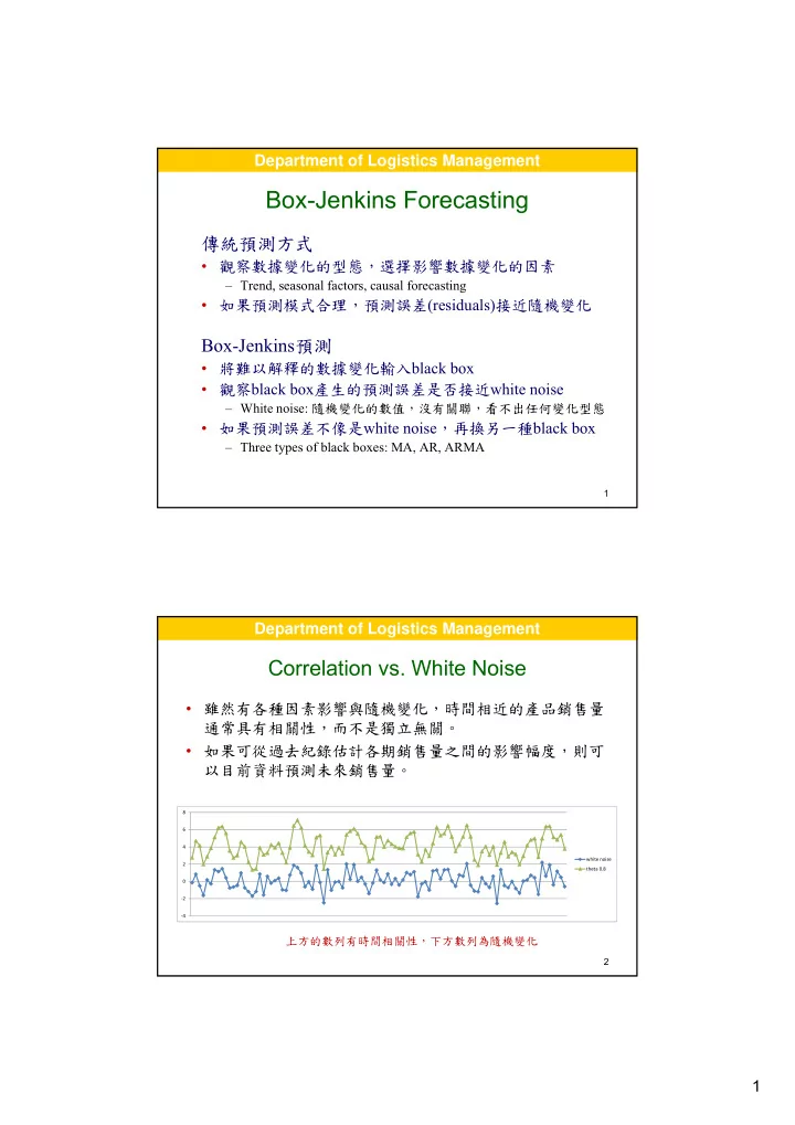
Correlation vs. White Noise

  • 雖然有各種因素影響與隨機變化,時間相近的產品銷售量

通常具有相關性,而不是獨立無關。

  • 如果可從過去紀錄估計各期銷售量之間的影響幅度,則可

以目前資料預測未來銷售量。

‐4 ‐2 2 4 6 8 white noise theta 0.8

2

上方的數列有時間相關性,下方數列為隨機變化

slide-2
SLIDE 2

2 Department of Logistics Management

Correlation Between Random Variables

  

1      n y y x x s

i i XY

x y

cov(x,y) corr(x,y)    correlation covariance cov(X, Y)=E[X-E(X)][Y-E(Y)]

衡量兩個隨機現象或 兩組數據間共同變化 的程度

  • 1 ≤ corr(x, y) ≤ 1
  • 1. cov(X, X)=Var(X)
  • 2. If X and Y are independent, then cov(X,Y)=E(XY)-E(X)E(Y)=0

cov(X, Y)≈

兩組數據間 的相關係數 標準化,不受X, Y大小的影響

3

  

  

  

    

n i i n i i n i i i

y y x x y y x x Y X

1 2 1 2 1

) ( ) ( ) , ( 

Department of Logistics Management

  • I. Autocorrelation

t t t t

(t, ) cov(y ,y ) E(y )(y )

 

        (t, ) ( )     

t t t

(0) cov(y ,y ) var(y )     

t t t t

cov(y , y ) ( ) ( ) ( ) (0) var(y ) var(y ) (0) (0)

 

           

autocovariance covariance stationary Autocorrelation

(只與時間差距有關,與時間t無關)

同一組銷售數據,時間相近的銷售量可能具有相關性

標準化,不受單位轉換的影響

4

slide-3
SLIDE 3

3 Department of Logistics Management

Estimating Autocorrelation

 

 

   

    

T t t T t t t

y y T y y y y T

1 2 1

) ( 1 ) )( ( 1 ) ( ˆ

 

  

T t t 1

1 y y T

 

t t 2 t

E (y ) (y ) ( ) E[(y ) ]



        

  

  

 

   

t t t

y y c y ˆ ˆ ˆ ˆ

1 1

Partial Autocorrelation =1, 2, 3, …

考慮其他各期也在同時影響

5

Department of Logistics Management

A Simple Example of Autocorrelation

6

slide-4
SLIDE 4

4 Department of Logistics Management

Autocorrelation Function

gradual damped oscillation

  • ne-sided gradual damping

觀察各個autocorrelation的大小,以挑選適合的 black box: MA, AR, ARMA models

7

Department of Logistics Management

隨機擲銅板,正面贏$1,反面輸$1,觀察累積金額

8

slide-5
SLIDE 5

5 Department of Logistics Management

Computing Autocorrelations on MINITAB

Lag Autocorrelation 65 60 55 50 45 40 35 30 25 20 15 10 5 1 1.0 0.8 0.6 0.4 0.2 0.0

  • 0.2
  • 0.4
  • 0.6
  • 0.8
  • 1.0

Autocorrelation Function for winnings

(with 5% significance limits for the autocorrelations)

significance level

9

Department of Logistics Management

No Autocorrelations for White Noise

White noise~N(0, 2): 隨機變化,相鄰數值沒有關聯

white noise process Autocorrelation of white noise

Lag Autocorrelation 50 45 40 35 30 25 20 15 10 5 1 1.0 0.8 0.6 0.4 0.2 0.0

  • 0.2
  • 0.4
  • 0.6
  • 0.8
  • 1.0

Autocorrelation Function for white noise

(with 5% significance limits for the autocorrelations) I ndex white noise 200 180 160 140 120 100 80 60 40 20 1 3 2 1

  • 1
  • 2
  • 3

Time Series Plot of white noise

10

slide-6
SLIDE 6

6 Department of Logistics Management

Example: Canadian Employment Index

0.1 0.2 0.3 0.4 0.5 0.6 0.7 0.8 0.9 1 1 2 3 4 5 6 7 8 9 10 11 12

Quarterly index form 1962.1~1993.4 Autocorrelations

11

Department of Logistics Management

Computing Autocorrelations of CANEMP

Lag Autocorrelation 30 25 20 15 10 5 1 1.0 0.8 0.6 0.4 0.2 0.0

  • 0.2
  • 0.4
  • 0.6
  • 0.8
  • 1.0

Autocorrelation Function for caemp

(with 5% significance limits for the autocorrelations)

12

slide-7
SLIDE 7

7 Department of Logistics Management

Computing Partial Autocorrelations

Lag Partial Autocorrelation 30 25 20 15 10 5 1 1.0 0.8 0.6 0.4 0.2 0.0

  • 0.2
  • 0.4
  • 0.6
  • 0.8
  • 1.0

Partial Autocorrelation Function for canemp

(with 5% significance limits for the partial autocorrelations)

13

Question: 如何挑選符合上一頁與本頁圖形的black box?

Department of Logistics Management

如果選擇適當的black box,預測誤 差(residual)應該接近white noise

觀察Autocorrelations與Partial Autocorrelations,以選擇適當 的black box

14

估計black box的參數

slide-8
SLIDE 8

8 Department of Logistics Management

  • II. Moving Average Models

The MA(1) Process yt = c + t + t-1 t is white noise

=0 → yt等於white noise >0 →數據呈現正相關

0.2 0.4 0.6 0.8 1 1.2 1.4 1.6 1.8 1 3 5 7 9 11 13 15 17 19 21 23 25 27 29 31 33 35 37 39 41 43 45 47 49 51 53 55 57 59 61 Whitenoise MA1

15

本期的誤差 上期的誤差

Department of Logistics Management

MA(q) Process

2 t

WN(0, )   

Lag Autocorrelation 10 9 8 7 6 5 4 3 2 1 1.0 0.8 0.6 0.4 0.2 0.0

  • 0.2
  • 0.4
  • 0.6
  • 0.8
  • 1.0

Autocorrelation Function for C3

(with 5% significance limits for the autocorrelations)

yt = c + t + t-1 + t-2 +…+ qt-q

MA(2) 1>0, 2>0 MA(2) 1<0, 2>0

Lag Autocorrelation 10 9 8 7 6 5 4 3 2 1 1.0 0.8 0.6 0.4 0.2 0.0

  • 0.2
  • 0.4
  • 0.6
  • 0.8
  • 1.0

Autocorrelation Function for C3

(with 5% significance limits for the autocorrelations)

顯著的項目數≈q

16

slide-9
SLIDE 9

9 Department of Logistics Management

Autocorrelation and Partial Autocorrelation

  • f MA processes

MA process: autocorrelation 圖形前幾段較顯著,partial autocorrelation為漸進式降低

17

Department of Logistics Management

Select MA(4) as Black Box for CANEMP

18

slide-10
SLIDE 10

10 Department of Logistics Management

Residual Plot of MA(4) Model for CANEMP

yt = 99.926 + t-1 + t-2 + t-3+ t-4 + t

Index Data Residual 117 104 91 78 65 52 39 26 13 1 120 110 100 90 80 70 60 50 40 20 15 10 5

  • 5
  • 10

Variable CANEMP Residual Fitted value

Time Series Plot of CANEMP, Residual, Fitted value 19

Department of Logistics Management

Autocorrelations of Residuals

  • 如果MA(4)模式合宜,residuals應該接近white noise,

而且沒有明顯的autocorrelations

Lag Autocorrelation 30 25 20 15 10 5 1 1.0 0.8 0.6 0.4 0.2 0.0

  • 0.2
  • 0.4
  • 0.6
  • 0.8
  • 1.0

Autocorrelation Function for RESMA(4)

(with 5% significance limits for the autocorrelations)

20

slide-11
SLIDE 11

11 Department of Logistics Management

  • III. Autoregressive Models

2 t

WN(0, )    The AR(1) Process

1 2 3 4 5 6 7 1 11 21 31 41 51 61 71 81 91 101 111 121 131 141 151 161 171 181 191 AR1 AR2

21

yt = ϕ1 yt-1 + t

The AR(2) Process

yt = ϕ1 yt-1 + ϕ2 yt-2 + t

上期的銷售 本期的誤差

Department of Logistics Management

Autocorrelations of AR(1) Process

=0.4 =0.95

0.1 0.2 0.3 0.4 0.5 0.6 0.7 0.8 0.9 1 1 2 3 4 5 6 7 8 9 10 11 12

What if <0?

22

slide-12
SLIDE 12

12 Department of Logistics Management

AR(p) Process

2 t

WN(0, )   

AR(2)

Lag Autocorrelation 24 22 20 18 16 14 12 10 8 6 4 2 1.0 0.8 0.6 0.4 0.2 0.0

  • 0.2
  • 0.4
  • 0.6
  • 0.8
  • 1.0

Autocorrelation Function for AR(2)

(with 5% significance limits for the autocorrelations) Lag Partial Autocorrelation 24 22 20 18 16 14 12 10 8 6 4 2 1.0 0.8 0.6 0.4 0.2 0.0

  • 0.2
  • 0.4
  • 0.6
  • 0.8
  • 1.0

Partial Autocorrelation Function for AR(2)

(with 5% significance limits for the partial autocorrelations)

23

yt = ϕ1 yt-1 + ϕ2 yt-2 + … + ϕp yt-p + t

Department of Logistics Management

Partial autocorrelations: , 1 p( ) 0, 1             Autocorrelations:

 , 3 , 2 , 1 ) (      

Autocorrelation and Partial Autocorrelation

  • f AR Processes

24

slide-13
SLIDE 13

13 Department of Logistics Management

Residual Plot of AR(2) Model for CANEMP

yt = 2.2382 + 1.5235yt-1  0.5463yt-2 + t

Time Data Residual2 117 104 91 78 65 52 39 26 13 1 120 110 100 90 80 70 60 50 40 20 15 10 5

  • 5
  • 10

Variable CANEMP Residual2 Fitted 2

Time Series Plot of CANEMP, Residual2, Fitted 2

25

Department of Logistics Management

AR(2) Model Residual Sample Autocorrelation

Lag Autocorrelation 30 25 20 15 10 5 1 1.0 0.8 0.6 0.4 0.2 0.0

  • 0.2
  • 0.4
  • 0.6
  • 0.8
  • 1.0

Autocorrelation Function for RESAR(2)

(with 5% significance limits for the autocorrelations)

  • Residuals沒有明顯的autocorrelations,AR(2)為合宜模式

26

slide-14
SLIDE 14

14 Department of Logistics Management

  • IV. Making Forecasts

27

Department of Logistics Management

Forecasts of MA(4) Model

Time canemp 140 130 120 110 100 90 80 70 60 50 40 30 20 10 1 115 110 105 100 95 90 85 80

Time Series Plot for canemp

(with forecasts and their 95% confidence limits)

Period Forecast Lower Upper 137 93.281 89.545 97.016 138 95.726 88.404 103.048 139 98.098 88.084 108.111 140 99.705 88.516 110.894 141 99.926 88.540 111.312 142 99.926 88.540 111.312 143 99.926 88.540 111.312 144 99.926 88.540 111.312 145 99.926 88.540 111.312 146 99.926 88.540 111.312

28

An MA(q) process is not forecastable more than q steps ahead. 根據先前的預測誤差來調整預測

yt = 99.926 +  t-1 + t-2 + t-3+ t-4 + t

slide-15
SLIDE 15

15 Department of Logistics Management

Forecasts of AR(2) Model

Time canemp 140 130 120 110 100 90 80 70 60 50 40 30 20 10 1 115 110 105 100 95 90 85 80

Time Series Plot for canemp

(with forecasts and their 95% confidence limits)

Period Forecast Lower Upper 137 92.341 89.539 95.144 138 92.651 87.544 97.759 139 92.946 85.817 100.075 140 93.225 84.375 102.075 141 93.490 83.187 103.792 142 93.740 82.214 105.266 143 93.977 81.416 106.538 144 94.201 80.760 107.643 145 94.413 80.219 108.607 146 94.614 79.773 109.455

29

yt = 2.2382 + 1.5235yt-1  0.5463yt-2 + t

根據先前的實際銷售量來調整預測 根據先前的預測值來調整預測

Department of Logistics Management

  • V. AutoRegressive Moving Average Models

t~WN(0, 2)

yt= yt-1+t ARMA(1,1) yt = c + t + t-1

yt = c + yt-1+ t + t-1

t~WN(0, 2)

ARMA(p,q)

yt = c+1yt-1+…+ pyt-p+ t + t-1+… + qt-q

30

AR(1) MA(1) 前幾期的銷售與前幾期的誤差都有影響

slide-16
SLIDE 16

16 Department of Logistics Management

Autocorrelations of ARMA Models

Partial Autocorrelations Autocorrelations AR(p) dies off truncates after lag p MA(q) truncates after lag q dies off ARMA(p,q) dies off dies off

31

Department of Logistics Management

Identify the Order of AR and MA

32

Autocorrelations Partial Autocorrelations

  • p=partial autocorrelations明顯大於0的lags數目
  • q=autocorrelations明顯大於0的lags數目
  • Trial and error: p=0, 1, 2, q=0, 1, 2
slide-17
SLIDE 17

17 Department of Logistics Management

Autocorrelations and Partial Autocorrelations

  • f CANEMP

33

Lag Autocorrelation 30 25 20 15 10 5 1 1.0 0.8 0.6 0.4 0.2 0.0

  • 0.2
  • 0.4
  • 0.6
  • 0.8
  • 1.0

Autocorrelation Function for caemp

(with 5% significance limits for the autocorrelations) Lag Partial Autocorrelation 30 25 20 15 10 5 1 1.0 0.8 0.6 0.4 0.2 0.0

  • 0.2
  • 0.4
  • 0.6
  • 0.8
  • 1.0

Partial Autocorrelation Function for canemp

(with 5% significance limits for the partial autocorrelations)

Department of Logistics Management

ARMA(2,4) Model for CANEMP

34

126 112 98 84 70 56 42 28 14 1 115 110 105 100 95 90 85 80 Index Data

canemp FITS4 Variable

Time Series Plot of ARMA(2,4)

30 25 20 15 10 5 1 1.0 0.8 0.6 0.4 0.2 0.0

  • 0.2
  • 0.4
  • 0.6
  • 0.8
  • 1.0

Lag Autocorrelation

Autocorrelation Function for ARMA(2,4) Residuals

(with 5% significance limits for the autocorrelations) 30 25 20 15 10 5 1 1.0 0.8 0.6 0.4 0.2 0.0

  • 0.2
  • 0.4
  • 0.6
  • 0.8
  • 1.0

Lag Partial Autocorrelation

Partial Autocorrelation Function for ARMA(2,4) Residuals

(with 5% significance limits for the partial autocorrelations)

slide-18
SLIDE 18

18 Department of Logistics Management

ARMA(3,1) Model for CANEMP

Index Data RESI3 126 112 98 84 70 56 42 28 14 1 120 110 100 90 80 70 60 50 40 15 10 5

Variable RESI3 canemp FITS3

Time Series Plot of canemp, FITS3, RESI3

Final Estimates of Parameters Type Coef SE Coef T AR 1 1.7894 0.8564 2.09 AR 2 -0.8998 1.2738 -0.71 AR 3 0.0950 0.4386 0.22 MA 1 0.3752 0.8455 0.44 Constant 1.51722 0.07907 19.19

35

Department of Logistics Management

  • VI. Nonstationary Time Series

A time series may have trend or changing variability over time. 不同期銷售量 yt+h 與 yt 的關聯受時間差h影響,也受時刻t影響

36

1 2 3 4 5 6 1 4 7 10 13 16 19 22 25 28 31 34 37 40 43 46 49 52 55 58 61 64 67 70 73 76 79 82 85 88 91 94 97 100

1 2 3 4 5 6 1 4 7 10 13 16 19 22 25 28 31 34 37 40 43 46 49 52 55 58 61 64 67 70 73 76 79 82 85 88 91 94 97 100

slide-19
SLIDE 19

19 Department of Logistics Management

37

‐10 ‐5 5 10 15 20 25 30 35 1 51 101 151 201 251 301 351 401

winnings

隨機擲銅板,正面贏$1,反面輸$1,觀察累積金額

銅板出現正面的機率=0.51,累積金額隨實驗次數增加而成長

Department of Logistics Management

Estimating Trends with Differences

1

2 1

 

 

T Y Y

T t t t

First Difference=Yt − Yt-1 1

2 1

 

 

T Y Y

T t t t

=0.037 ≈ E[winning]=10.51+(-1)0.49=0.02

Trend≈ 如果觀察到非線性的趨勢 Use Second Difference=(Yt − Yt-1) − (Yt-1 − Yt-2) to estimate nonlinear trends

38

slide-20
SLIDE 20

20 Department of Logistics Management

Autoregressive Integrated Moving Average

ARIMA(p, d, q)

AR(p) MA(q)

An ARIMA(0,1,1) model is single exponential smoothing

Number of differences

ARIMA(p,0,0)=AR(p), ARIMA(0,0,q)=MA(q), ARIMA(p,0,q)=ARMA(p,q)

zt=t + 1t-1 zt=Yt − Yt-1  Yt = Yt-1+ zt = Yt-1+ t + 1t-1 ≈ Yt-1+ 1t-1

39

Department of Logistics Management

Analyzing Apparel Sales data

Index Sales 100 90 80 70 60 50 40 30 20 10 1 20.0 17.5 15.0 12.5 10.0 7.5 5.0

Time Series Plot of Sales

Lag Autocorrelation 24 22 20 18 16 14 12 10 8 6 4 2 1.0 0.8 0.6 0.4 0.2 0.0

  • 0.2
  • 0.4
  • 0.6
  • 0.8
  • 1.0

Autocorrelation Function for Sales

(with 5% significance limits for the autocorrelations) Lag Partial Autocorrelation 24 22 20 18 16 14 12 10 8 6 4 2 1.0 0.8 0.6 0.4 0.2 0.0

  • 0.2
  • 0.4
  • 0.6
  • 0.8
  • 1.0

Partial Autocorrelation Function for Sales

(with 5% significance limits for the partial autocorrelations)

40

slide-21
SLIDE 21

21 Department of Logistics Management

ARIMA(1,0,0)=AR(1)

Index Data 100 90 80 70 60 50 40 30 20 10 1 20 15 10 5

Variable FITS1 Sales RESI1

Time Series Plot of Sales, RESI1, FITS1 41

Department of Logistics Management

Compute the First Differences

Index C5 100 90 80 70 60 50 40 30 20 10 1 3 2 1

  • 1
  • 2
  • 3

Time Series Plot of First Differences

Lag Autocorrelation 24 22 20 18 16 14 12 10 8 6 4 2 1.0 0.8 0.6 0.4 0.2 0.0

  • 0.2
  • 0.4
  • 0.6
  • 0.8
  • 1.0

Autocorrelation Function for Difference

(with 5% significance limits for the autocorrelations) Lag Partial Autocorrelation 24 22 20 18 16 14 12 10 8 6 4 2 1.0 0.8 0.6 0.4 0.2 0.0

  • 0.2
  • 0.4
  • 0.6
  • 0.8
  • 1.0

Partial Autocorrelation Function for Difference

(with 5% significance limits for the partial autocorrelations)

42

First Difference=Yt − Yt-1

slide-22
SLIDE 22

22 Department of Logistics Management

ARIMA(1,1,0)

43

I ndex Data 100 90 80 70 60 50 40 30 20 10 1 20.0 17.5 15.0 12.5 10.0 7.5 5.0

Variable Sales FITS3

Time Series Plot of Sales, ARI MA(1,1,0)

Department of Logistics Management

Lag Autocorrelation 24 22 20 18 16 14 12 10 8 6 4 2 1.0 0.8 0.6 0.4 0.2 0.0

  • 0.2
  • 0.4
  • 0.6
  • 0.8
  • 1.0

Autocorrelation Function for Residuals of ARI MA(1,1,0)

(with 5% significance limits for the autocorrelations)

Compare Autocorrelations of Errors

ARIMA(1,1,0)

44

Lag Autocorrelation 24 22 20 18 16 14 12 10 8 6 4 2 1.0 0.8 0.6 0.4 0.2 0.0

  • 0.2
  • 0.4
  • 0.6
  • 0.8
  • 1.0

Autocorrelation Function for ARIMA(1,0,0) Residuals

(with 5% significance limits for the autocorrelations)

ARIMA(1,0,0)

slide-23
SLIDE 23

23 Department of Logistics Management

24 22 20 18 16 14 12 10 8 6 4 2 1.0 0.8 0.6 0.4 0.2 0.0

  • 0.2
  • 0.4
  • 0.6
  • 0.8
  • 1.0

Lag Partial Autocorrelation

Partial Autocorrelation Function for ARIMA(1,0,0) Residuals

(with 5% significance limits for the partial autocorrelations)

Compare Partial Autocorrelations of Errors

Lag Partial Autocorrelation 24 22 20 18 16 14 12 10 8 6 4 2 1.0 0.8 0.6 0.4 0.2 0.0

  • 0.2
  • 0.4
  • 0.6
  • 0.8
  • 1.0

Partial Autocorrelation Function for Residuals of ARI MA(1,1,0)

(with 5% significance limits for the partial autocorrelations)

45

ARIMA(1,0,0) ARIMA(1,1,0)

Department of Logistics Management

ARIMA(0,1,1)=exponential smoothing

Index Data 100 90 80 70 60 50 40 30 20 10 1 20 15 10 5

Variable FITS2 Sales RESI2

Time Series Plot of ARIMA(0,1,1)

46

24 22 20 18 16 14 12 10 8 6 4 2 1.0 0.8 0.6 0.4 0.2 0.0

  • 0.2
  • 0.4
  • 0.6
  • 0.8
  • 1.0

Lag Partial Autocorrelation

Partial Autocorrelation Function for ARIMA(0,1,1) Residuals

(with 5% significance limits for the partial autocorrelations) Lag Autocorrelation 24 22 20 18 16 14 12 10 8 6 4 2 1.0 0.8 0.6 0.4 0.2 0.0

  • 0.2
  • 0.4
  • 0.6
  • 0.8
  • 1.0

Autocorrelation Function for ARIMA(0,1,1) Residuals

(with 5% significance limits for the autocorrelations)

slide-24
SLIDE 24

24 Department of Logistics Management

Forecast performance and accuracy

  • Forecast accuracy is a function of

– forecast horizon 短期預測比較準確 – level of aggregation 總合預測比單一品項或單一地區的預測準確 – product maturity 民生需求的預測比較準確

  • Frequency of monitoring depends on importance
  • Combining the results of forecasting methods yields

better forecasts

  • Improving forecasting accuracy is not the only solution

– it may be easier to buffer against or reduce uncertainty

47