C C C general form for Versatile Non-linear model of - - PowerPoint PPT Presentation

SLIDE 1

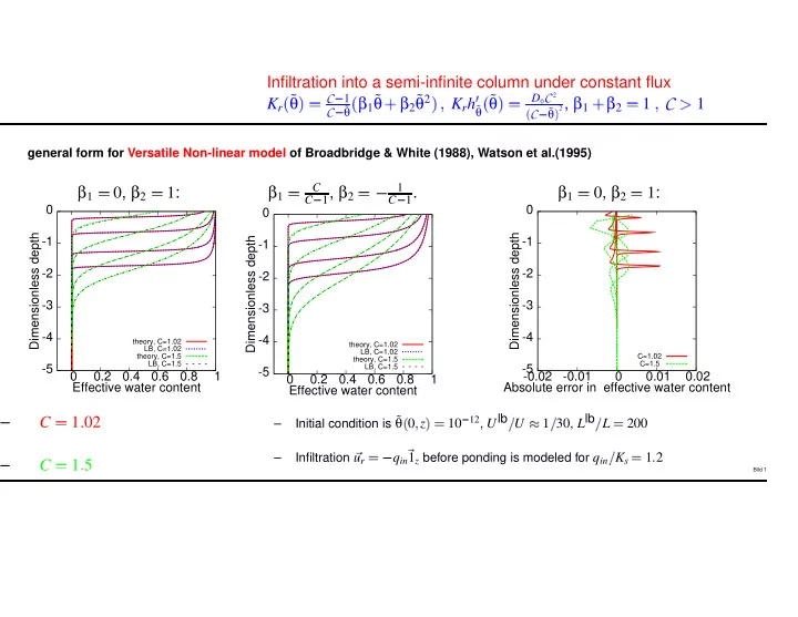
Infiltration into a semi-infinite column under constant flux Kr

• ˜

θ

✁ ✂

C

✄

1

C

✄

˜ θ

• β1˜

θ

☎

β2˜ θ2

✁ ✆

Krh

✝

˜ θ

• ˜

θ

✁ ✂

D0C 2

✞

C

✄

˜ θ

✟

2, β1

☎

β2

✂

1

✆

C

✠

1

general form for Versatile Non-linear model of Broadbridge & White (1988), Watson et al.(1995)

β1

✂

C C

✄

1, β2

✂ ✡

1 C

✄

1.

• 5
• 4
• 3
• 2
• 1

0.2 0.4 0.6 0.8 1 Dimensionless depth Effective water content

theory, C=1.02 LB, C=1.02 theory, C=1.5 LB, C=1.5

β1

✂

0, β2

✂

1:

• 5
• 4
• 3
• 2
• 1
• 0.02
• 0.01

0.01 0.02 Dimensionless depth Absolute error in effective water content

C=1.02 C=1.5

β1

✂

0, β2

✂

1:

• 5
• 4
• 3
• 2
• 1

0.2 0.4 0.6 0.8 1 Dimensionless depth Effective water content

theory, C=1.02 LB, C=1.02 theory, C=1.5 LB, C=1.5

– C

✂

1

☛

02 – C

✂

1

☛

5

– Initial condition is ˜

θ

☞ ✌

z

✍✏✎

10

✑

12, Ulb

✒

U

✓

1

✒

30, Llb

✒

L

✎

200

– Infiltration

✔

ur

✎ ✕

qin

✔

1z before ponding is modeled for qin

✒

Ks

✎

1

✖

2

Bild 1

SLIDE 2

Steady state infiltration with VGM (van Genuchten 1980) and modified VGM (Vogel et al. 2001) models: ˜ θ

• h

✁ ✂

β0

• 1

☎

• ✡

α0h

✁

n

✁ ✄

m, β0

✂

• 1

☎

• ✡

α0hs

✁

n

✁

m,

α0

✠

0, n

✠

1 and m

✂

1

✡

1

• n as empirical parameters

Without averaging

2 4 6 8 10

• 0.5 0 0.5 1 1.5 2 2.5 3 3.5

Vertical coordnate z, [m] Pressure head h, [m]

Moisture formulation, h_s=0 Darcy, h_s=0 Moisture formulation, h_s=-9cm Darcy

With averaging

1 2 3 4 5 6 7 8 9 10

• 0.5 0 0.5 1 1.5 2 2.5 3 3.5

Vertical coordnate z, [m] Pressure head h, [m]

Moisture form.+Averaging, h_s=0 Darcy, h_s=0

– Original model: h

✝

˜ θ

• hs

✁

is unbounded, hs

✂

– Modified model: h

✝

˜ θ

• hs

✁

is bounded, hs

✁

– Example: Sandy soil, α

✂

3

☛

7m

✄

1, n

✂

5

• 0.1
• 0.08
• 0.06
• 0.04
• 0.02

0.999 0.9992 0.9994 0.9996 0.9998 1

Pressure head h, [m] Effective water content

h_s=0 h_s=-3cm h_s=-9cm

red : hs

✂

green: hs

✂ ✡

3 cm blue : hs

✂ ✡

9 cm

– Input flux is qin

✎ ✖

1Ks, Ks

✎ ✖

1m

✒

h, h

☞

zL

✎ ✍ ✎

3

✖

4 m. Box has 100 cells.

Bild 2

SLIDE 3

Exact variably saturated non-stationary solution

J.-P. Carlier (Cemagref, 2004) following “A class of exact solutions for Richards’ equation”, Barry et al.(1993)

• 1.6
• 1.5
• 1.4
• 1.3
• 1.2
• 1.1
• 1
• 0.9
• 0.8
• 0.7
• 0.6
• 4.5
• 4
• 3.5
• 3
• 2.5
• 2
• 1.5
• 1
• 0.5
• Depth Z, m

Pressure head, m

theory LB 0.05 0.1 0.15 0.2 0.25 0.3 0 100 200 300 400 500 600 700 800 900 1000

Relative L^2-Error Time, h

sub_it=0 sub_it=5 sub_it=10 sub_it=50 sub_it=1000

– Exact h

☞

t

✍

• solution is fixed at top Z

✎ ✖

6m and the bottom Z

✎

1

✖

6 m

– Computations are started at t

✎

t0

✎ ✖

1h, h

☞

t0

✌

Z

✎

1

✖

6 m

✍ ✎ ✕

72m

– Picture: t

✎

20

✖ ✖ ✖

103 h

a) Definition of retention curve: ˜ θ

• h

✁ ✂

γ

• h

✄

∞ 1 h

✁ ✂

B∂h

✁

Krdh

✝

γ

✄

1

✂

• hs

✄

∞ 1 h

✁ ✂

B∂h

✁

Krdh

✝

b) BCM hydraulic conductivity function: Kr

• h

✁ ✂

• h
• hs

✁ ✄

β,

B

✂

0 then h

• ˜

θ

✁ ✂

hs˜ θ

✄

1

✄ ✞

β

✂

1

✟

c) Linear solution within both zones: h

✂

Z A

✞

t

✟ ✆

h

• t

✆ ✁ ✂ ✆

A

• t

✁ ✂

1

☎

W

☎ ✡

e

✞

tKs

✆

θs

✝

θr

✞

γ

✄

1

✟ ✟ ✆

with Lambert function W

• x

✁

, x

✂

W

• x

✁

exp

☎

W

• x

✁ ✟

.

Bild 3

SLIDE 4

Steady state infiltration in Sandy soil using h

✡

and θ

• h

✡

formulations: Pressure head formulation

1 2 3 4 5 6 7 8 9 10

• 0.5 0 0.5 1 1.5 2 2.5 3 3.5

Vertical coordnate z, [m] Pressure head h, [m]

Pressure formulation, h_s=0 Darcy, h_s=0

Mixed formulation

1 2 3 4 5 6 7 8 9 10

• 0.5 0 0.5 1 1.5 2 2.5 3 3.5

Vertical coordnate z, [m] Pressure head h, [m]

Mixed formulation, h_s=0 Darcy

• Pressure head formula-

tion does not use re- tention curves and has no approximation when h

✝

˜ θ

• hs

✁

is unbounded, hs

✂

0.

• Mixed formulation does

not use retention cur- ves in unsaturated zone but needs h

✝

˜ θ

• 1

✁

to ex- trapolate them beyond air entry value hs. He- re, P

✂

h

✝

˜ θ

• 1

✡

10

✄

6

✁ ✂

3566

☛

24 m.

– Pressure head hL is fixed to 3

✖

4 m at the bottom zL

✎

0.

– Input flux is qin

✎ ✖

• 1Ks. Box has 100 cells.

Bild 4

SLIDE 5

Dispersion relation (D.d’Humières)

• Solution is looked in the form,

f

✂

f 0exp

• i

☎

• k

✁

• r

✡

• Ut

✁ ✡

ωt

✟ ✁

, where ω

• k

✁ ✂ ✡

iν

• k

✁

k2 ν

• k

✁ ✂

∑α

✂

βDαβ kαkβ k2

• k

✂

• kx

✆

ky

✆

kz

✁ ✂

k

• cosθsinφ

✆

sinθsinφ

✆

cosφ

✁

.

• z

✂

exp

• ✡

iωt

✁

and f 0 are the eigenvalues and eigenvectors

• f the linear operator

✄ ✄

1

✁ ✆☎ ☎ ✝ ✁ ✆☎ ✡ ✞

eq.

✁ ✁

, f eq.

✂ ✞

eq.

✁

f

✄ ✂

diag

• exp
• k

✁

• Cj

✁ ✁

– Diffusion term: νlb

• k

✁ ✂

ν

• k

✁

• 1

☎

ν

✞

r

✟

1

• k

✁

k2

☎ ✁ ✁ ✁ ☎

ν

✞

r

✟

n

• k

✁

k2n

☎ ✁ ✁ ✁ ✁

– Optimal diffusion solution ν

✞

r

✟

1

• k

✁ ✂

0 for any

• k, c2

s and a

✞

e

✟

is Λ2

• λopt

D

✆

λopt

e

✁ ✂

2 9

✆

λopt

D

✂ ✡

3

☎ ✟

3

✆

– Advection term:

• k

✁

• Ulb

✂

• k

✁

• U
• 1

☎

u

✞

r

✟

1

• k

✁

k2

☎ ✁ ✁ ✁ ☎

u

✞

r

✟

n

• k

✁

k2n

☎ ✁ ✁ ✁ ✁

– Optimal advection solution u

✞

r

✟

1

• k

✁ ✂

0 is BGK Model Λ2

• λopt

D

✆

λopt

e

✁ ✂

1 9

✆

λopt

D

✂

λopt

e

✂ ✡

3

☎ ✟

3

Bild 5