Causation as Production and Dependence or, A Model-Invariant Tieory - - PDF document

Causation as Production and Dependence

• r, A Model-Invariant Tieory of Causation
• J. Dmitri Gallow

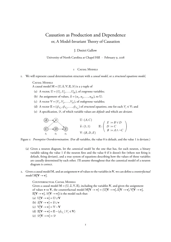
University of North Carolina at Chapel Hill · February 9, 2018 1 Causal Models 1. We will represent causal determination structure with a causal model, or a structural equations model, Causal Models A causal model = (, ⃗ u,,,) is a 5-tuple of (a) A vector, = (U1,U2,...,UM ), of exogenous variables; (b) An assignment of values, ⃗ u = (u1, u2,..., uM ), to ; (c) A vector = (V1,V2,...,VN ), of endogenous variables; (d) A vector = (ϕV1,ϕV2,...,ϕVN ) of structural equations, one for each Vi ∈ ; and (e) A specifjcation, , of which variable values are default and which are deviant.

B

: (A,C ) ⃗ u : (1,1) : (B, D, E ) :   E := B ∨ D D := C B := A ∧ ¬C   Figure 1: Preemptive Overdetermination. (For all variables, the value 0 is default, and the value 1 is deviant.) (a) Given a neuron diagram, let the canonical model be the one that has, for each neuron, a binary variable taking the value 1 if the neuron fjres and the value 0 if it doesn’t fjre (where not fjring is default, fjring deviant), and a true system of equations describing how the values of those variables are causally determined by each other. I’ll assume throughout that the canonical model of a neuron diagram is correct. 2. Given a causal model , and an assignment v of values to the variables in V, we can defjne a counterfactual model [V → v]. Counterfactual Causal Models Given a causal model = (, ⃗ u,,), including the variables V, and given the assignment

• f values v to V, the counterfactual model [V → v] = ([V → v], ⃗

u[V → v],[V → v], [V → v], [V → v]) is the model such that: (a) [V → v] = ∪ V (b) ⃗ u[V → v] = ⃗ u ∪ v (c) [V → v] = − V (d) [V → v] = − (ϕVi | Vi ∈ V) (e) [V → v] = 1

3. Using counterfactual models, we may provide a semantics for causal counterfactuals: Causal Counterfactuals In a causal model , containing the variables in V, the causal counterfactual V = v → ψ is true ifg ψ is true in the counterfactual model [V → v], |= V = v → ψ ⇐⇒ [V → v] |= ψ 2 Model Invariance 4. Ideally, a theory of causation would satisfy the following principle: Model Invariance Given any two causal models, and †, which both contain the variables C and E , if both and † are correct, then C = c caused E = e in ifg C = c caused E = e in †. 5. In general, if = (, ⃗ u,,,) is a causal model with U ∈ , then let −U be the model that you get by: (a) Removing U from (b) Removing U ’s value from ⃗ u (c) Exogenizing any variables in whose only parent was U (d) Replacing U for its value in every structural equation in (e) Removing default information about U from . 6. If every equation in −U is surjective, then say that U is an inessential variable. Tien, we should endorse the following principle: Exogenous Reduction If a causal model = (, ⃗ u,,,) is correct, and U ∈ is inessential, then −U is also correct. 7. In general, if = (, ⃗ u,,,) is a causal model with V ∈ , then let −V be the model that you get by: (a) Leaving alone (b) Leaving ⃗ u alone (c) Removing V from (d) Removing ϕV from , and replacing V with ϕV (PA(V )) wherever V appears on the right-hand-side

• f an equation in 1

(e) Removing default information about V from 8. (a) If V has a single parent, Pa, and a single child, C h, and if Pa is not also a parent of C h, then say that V is an interpolated variable. ... Pa → V → C h ... (b) If V is interpolated and all the equations in −V are surjective, then say that V is inessential. (c) Tien, we should accept the following principle: Endogenous Reduction If a causal model = (, ⃗ u,,,) is correct, and V ∈ is an inessential variable, then −V is also correct. 9. Tiough there isn’t the space to show it here, the accounts of Hitchcock (2001, 2007), Halpern & Pearl (2001, 2005), Woodward (2003), Halpern (2008), and Weslake (forthcoming) are all inconsistent with Model Invariance, Exogenous Reduction, and Endogenous Reduction.

1

PA(E ) are E ’s causal parents in the model—those variables which appear on the right-hand-side of E ’s structural equation ϕE .

2

B

: (A,C ) ⃗ u : (1,1) : (B, E ) : E := B ∨ C B := A ∧ ¬C

• Figure 2: Preemptive Overdetermination

3 A Model Invariant Theory of Causation

• 10. I will present a theory of causation, formulated within the framework of structural equations models,

which is consistent with Endogenous Reduction, Exogenous Reduction, and Model Invariance. (a) I’ll build up the theory by progressing through some familiar cases from the literature. 3.1 Preemptive Overdetermination

• 11. (a) In the canonical model, 2, of Preemptive Overdetermination shown in fjgure 2, E = 1 does not

counterfactually depend upon C = 1. (b) However, if we just look at E ’s structural equation E := B ∨ C , and B and C ’s actual values, then E = 1 does counterfactually depend upon C = 1. Call this submodel of 2 the local model at E .

• 12. In general, we can defjne the local model at E as follows.

Local Causal Model Given a causal model = (, ⃗ u,,,), with E ∈ , the local model at E , ((E )), is the causal model in which (a) Tie exogenous variables are just the parents of E , PA(E ), in the original model ; (b) Tie exogenous variables PA(E ) are assigned the values they take on in ; (c) Tie sole endogenous variable is E ; (d) Tie sole structural equation is E ’s structural equation in , ϕE ; and (e) Tie defaults for E and PA(E ) are the same as in .

• 13. Say that E = e locally counterfactually depends upon C = c ifg, in the local model at E , ((E )), there’s

some c ∗, e∗ such that ((E )) |= C = c ∗ → E = e∗

• 14. A (preliminary) proposal, then, is that either local or global counterfactual dependence suffjces for cau-

sation. (a) While this helps with the case of preemptive overdetermination in fjgure 2, it does nothing to help with the neuron diagram from fjgure 1. (b) It would be nice to handle that case by appealing to the transitivity of causation. (c) Unfortunately, there are a number of counterexamples to the transitivity of causation. 3.2 Counterexamples to Transitivity

• 15. Sometimes, we can trace out of sequence of causal relations and conclude that the event at the start of

the chain caused the one at the end. If that’s so, then I’ll call the chain transitive. 3

A B

(a)

A C B

(b)

Figure 3: Tampering (cf. Paul & Hall 2013). Tie octogonal neurons can either fjre weakly (light grey) or strongly (dark grey). If C fjres, this diminishes the strength with which B fjres. In fjgure 3(a), C ’s fjring caused B to fjre weakly. And B’s fjring weakly caused E to fjre. But C ’s fjring didn’t cause E to fjre. (a) Lewis thought that causal chains were always transitive, but this has unpalatable consequences. Chris smokes, contracts cancer, undergoes chemo, and survives. Tie smoking causes the cancer; the cancer causes the chemo; and the chemo causes the survival—so Lewis is forced to say that the smoking causes the survival. (b) Tie right thing to say is that causal chains are sometimes, but not always, transitive. Tie diffjculty is working out just when.

• 16. Tie plan: I’ll attempt to give conditions specifying when a directed path, P, running from the variable

V1 to the variable VN , P = V1 → V2 → V3 → ··· → VN permits the inference that V1 = v1 caused VN = vN . When it does, I’ll call the path a transitive path.

• 17. One kind of counterexample to transitivity is illustrated by the neuron diagram in fjgure 3. C ’s fjring

caused B to fjre weakly (rather than strongly); B’s fjring weakly (rather than not) caused E to fjre. But C ’s fjring didn’t cause E to fjre.2 (a) Tie solution: adopt a contrastivist theory of causation, and require that the contrasts in our causal chain match up.3 (b) Note: once we go contrastivist, we will be theorizing in terms of a 4-place causal relation Cause(C = c,C = c ∗, E = e, E = e∗) From this, we may recover a familiar 2-place causal relation: Cause(C = c, E = e) ⇐⇒ ∃c ∗∃e∗Cause(C = c,C = c ∗, E = e, E = e∗)

• 18. For two other counterexamples to transitivity, consider the neuron diagrams in fjgure 4.

(a) In both cases, either the start or the end of the causal chain involves a default variable value. (b) Tiis suggests the hypothesis: in order for a directed path to be a transitive path, the variable values at the start and end of that path must both be deviant (and, though I won’t be motivating this requirement here, their contrasts must also be default).

• 19. In general, this will be our account of which a directed path in a causal model is transitive:

2

• Cf. McDermott (1995)’s Dog Bite example and the counterexamples to transitivity discussed in Paul (2004).

3

• cf. Schaffer (2005).

4

C

(a)

B E

(b)

Figure 4: In fjgure 4(a), C ’s failure to fjre causes B to fjre. B’s fjring causes E to fjre. But C ’s failure to fjre doesn’t cause E to fjre. In fjgure 4(b), C ’s fjring causes D to fjre. D’s fjring causes E to remain dormant. But C ’s fjring does not cause E to remain dormant. Figure 5: Short Circuit, again. C ’s fjring didn’t cause F to fjre, but without condition (c) of Transitive Path, we would have to say that it did. Transitive Path In a causal model , a directed path running from V1 to VN P = V1 → V2 → V3 → ··· → VN is a transitive path ifg: (a) For each variable Vi along P, there is a pair (vi, v∗

i ) of Vi’s actual value vi in , and a

contrast value v∗

i ,

(v1, v∗

1) → (v2, v∗ 2) → (v3, v∗ 3) → ··· → (vN , v∗ N )

such that: for all j between 1 and N − 1, Vj’s taking on the value vj, rather than v∗

j ,

caused Vj+1 to take on the value vj+1, rather than v∗

j+1;

(b) Both V1’s and VN ’s actual values are deviant, their contrast values default; and (c) Every departure variable along P causes each of its return variables along P.4 (a) To see the reason for this fjnal condition, consider the neuron diagram in fjgure 5. 3.3 Prevention and Omission without Dependence?

• 20. So far, we’ve only looked at causal relations where both the cause and efgect variables take on deviant
• values. But default variable values can also be causes and efgects.

(a) Because counterfactual dependence suffjces for causation, cases of prevention (fjgure 6) and omission (fjgure 7) involve default efgects and causes, respectively.

4

For any variables D, R along the path (unless (D, R) = (V1,VN )), D is a departure variable, and R is one of its return variables ifg there is a path, O = D → O1 → O2 → ··· → R, such that D and R are the only variables from P on O.

5

E Figure 6: Prevention C Figure 7: Omission

B E

(a)

B E D

(b)

B E

(c)

Figure 8: Prevention without Dependence?

• 21. When C = c and E = e were deviant variable values, we said that local counterfactual dependence was

suffjcient for causation. Should we say the same thing when C = c or E = e is a default variable value? (a) Tiis question turns out to be closely related to cases of Preemptive Prevention (or, cases of prevention without dependence) like the one shown in fjgure 8. (b) If we say that local counterfactual dependence suffjces for causation, then, in the canonical model of the neuron diagram in fjgure 8(a), we will say that C ’s fjring caused E to not fjre. (c) However, we would not be able to say the same thing about the neuron diagram in fjgure 8(b). For, in the canonical model of that neuron diagram, E = 0 does not locally counterfactually depend upon C = 1, since C isn’t even in the local model at E . Moreover, since E ’s remaining dormant is a default state of that neuron, we would not be able to appeal to the transitivity condition to say that C ’s fjring prevented E from fjring. (d) So, we should say that, in the case where the cause or efgect variable value is default, local counter- factual dependence is not suffjcient for causation, and therefore, in the cases shown in fjgure 8, C ’s fjring doesn’t prevent E from fjring all by itself.5

• 22. We can further support this treatment by noting that, if we want a model-invariant account of causation,

then we are forced to say, in fjgure 8(c), that C ’s fjring prevented E from fjring ifg D’s fjring also prevented E from fjring. (a) Beginning with the canonical causal model of fjgure 8(c), Exogenous Reduction allows us to remove the inessential exogenous variable A from our model. Tien, Endogenous Reduction allows us to remove the inessential interpolated variable B. We end up with a causal model containing the sole structural equation E := ¬C ∧ ¬D. But this equation treats C and D symmetrically, and both C and D take on the same value. So, any account of causation will say that, in this model, C = 1 caused E = 0 ifg D = 1 caused E = 0. Since D = 1 clearly did not cause E = 1, any model-invariant account of causation should say that C = 1 didn’t caused E = 0 either.

• 23. So there is no prevention without dependence. Can there be omission without dependence? For parallel

reasons, it does not appear so. Consider the neuron diagrams from fjgure 9.

5

We can still say that the disjunction of A’s fjring and C ’s fjring caused E to remain dormant.

6

C B

(a)

C D B

(b)

Figure 9: Omission without Dependence? (a) Suppose we said that local dependence suffjced for C = 0 causing E = 1 in fjgure 9(a). Tien, we should say the same thing about fjgure 9(b). However, in the canonical model of fjgure 9(b), there is no local dependence between E = 1 and C = 0. Moreover, there can be no transitive path running from C to E in that canonical model, since C ’s actual value is default.

• 24. Exactly similar issues arise when we consider cases of local dependence where both C and E ’s values are

default (left as an exercise). So we should conclude that local dependence suffjces for causation only when C and E both have deviant values (and default contrasts). 3.4 Causation as Production and Dependence

• 25. In summary, we have arrived at the following account of causation:

Causation as Production and Dependence In a causal model , C ’s taking on the value c, rather than c ∗, caused E to take on the value e, rather than e∗, ifg either (Prod) or (Dep). (Prod) Both c and e are deviant variable values, the contrasts c ∗ and e∗ defaults, and either: i. In the local model at E , ((E )), had C taken on the value c ∗, E would have taken

• n the value e∗,

M ((E )) |= C = c ∗ → E = e∗

• r
• ii. In , there is a transitive path leading from C to E .

(Dep) In , had C taken on the value c ∗, E would have taken on the value e∗, |= C = c ∗ → E = e∗

• 26. Tiis account is consistent with Model Invariance, Exogenous Reduction, and Endogenous Reduc-
• tion. Suppose that we have a correct model = (, ⃗

u,,,), with U ∈ and V ∈ . And suppose that neither U nor V are C or E , and both U and V are inessential. Tien: (a) If C = c caused E = e in , then C = c caused E = e in −U ; (b) If C = c caused E = e in , then C = c caused E = e in −V ; (c) If C = c didn’t cause E = e in , then C = c didn’t cause E = e in −U ; and (d) If C = c didn’t cause E = e in , then C = c didn’t cause E = e in −V .

• 27. (a) Tie clause (Prod), taken in isolation, does a reasonably good job of capturing a notion of causal
• production. According to it, production involves the local, uninterrupted propagation of deviant,

non-inertial states of afgairs (rather than default, inertial states of afgairs). 7

B D H

(a)

C

(b)

Figure 10: Double Prevention without Dependence. Figure 10(b) shows what would have happened, had C not fjred, in fjgure 10(a). (b) A hypothesis: the notion of causal production encapsulated in the Production clause of this account represents the core of our concept of causation. Tiose causal judgments which are licensed by the Production clause alone are far more intuitive, natural, and widespread than those which are only licensed with the addition of the Dependence clause. i. For instance, the Production clause is all that is required to show that C ’s fjring caused E to fjre in cases of Preemptive Overdetermination. And the judgment that C caused E in this case is widespread and uncontested.

• ii. In contrast, in order to establish causation in cases of prevention, omission, omissive prevention,

double prevention, and so on, we will need to appeal to the Dependence clause. And these judgments are all less uniform and more controversial. (c) However, if we accept the Production clause, then the full strength of the Dependence clause is re- quired, if we are to satisfy Model Invariance, Exogenous Reduction, and Endogenous Reduction. i. Consider, for instance, the neuron diagram shown in fjgure 10(a). I take it that it is far from clear what to say about whether C ’s fjring caused E to fjre in fjgure 10(a). But, by removing inessential variables, this neuron diagram may be reduced to the model of preemptive overdetermination from fjgure 1.

• ii. In the case of preemptive overdetermination, we must say that C = 1 caused E = 1 (by Prod).

So, if we wish our account to be model-invariant, then we must say that C = 1 caused E = 1 in the canonical model of fjgure 10(a).

• iii. But in order to conclude this with the transitivity clause, we must have C = 1 cause D = 0,

D = 0 cause H = 0, and H = 0 cause E = 1.

• iv. So, we must count as causal cases of prevention, omission, and omissive prevention. We must

appeal to the full strength of Dependence. 8

References Collins, John, Ned Hall & L. A. Paul, editors. 2004. Causation and Counterfactuals. Tie MIT Press, Cambridge,

• ma. [9]

Halpern, Joseph Y. 2008. “Defaults and Normality in Causal Structures.” Proceedings of the Eleventh International Conference on Principles of Knowledge Representation and Reasoning, 198–208. [2] —. 2016. Actual Causality. MIT Press, Cambridge, ma. Halpern, Joseph Y. & Christopher Hitchcock. 2010. “Actual Causation and the Art of Modeling.” In Heuristics, Probability and Causality: A Tribute to Judea Pearl, Rina Dechter, Hechtor Geffner & Joseph Y. Halpern, editors, 383–406. College Publications. —. 2015. “Graded Causation and Defaults.” Tie British Journal for the Philosophy of Science, vol. 66 (2): 413–457. Halpern, Joseph Y. & Judea Pearl. 2001. “Causes and Explanations: A Structural-Model Approach. Part 1: Causes.” In Proceedings of the Seventeeth Conference on Uncertainty in Artifjcial Intelligence, John Breese & Daphne Koller, editors, 194–202. Morgan Kaufman, San Francisco. [2] —. 2005. “Causes and Explanations: A Structural-Model Approach. Part 1: Causes.” Tie British Journal for the Philosophy of Science, vol. 56: 843–887. [2] Hitchcock, Christopher. 2001. “Tie Intransitivity of Causation Revealed in Equations and Graphs.” Tie Journal

• f Philosophy, vol. 98 (6): 273–299. [2]

—. 2007. “Prevention, Preemption, and the Principle of Suffjcient Reason.” Philosophical Review, vol. 116 (4): 495–532. [2] Lewis, David K. 2000. “Causation as Infmuence.” Tie Journal of Philosophy, vol. 97 (4): 182–197. Reprinted in Collins et al. (2004, pp. 75–106). [4] —. 2004. “Causation as Infmuence.” In Collins et al. (2004), chap. 3, 75–106. [4] McDermott, Michael. 1995. “Redundant Causation.” Tie British Journal for the Philosophy of Science, vol. 46 (4): 523–544. [4] McGrath, Sarah. 2005. “Causation by Omission: A Dilemma.” Philosophical Studies, vol. 123: 125–148. Paul, L. A. 2004. “Aspect Causation.” In Collins et al. (2004). [4] Paul, L. A. & Ned Hall. 2013. Causation: A User’s Guide. Oxford University Press, Oxford. [4] Schaffer, Jonathan. 2005. “Contrastive Causation.” Tie Philosophical Review, vol. 114 (3): 297–328. [4] Weslake, Brad. forthcoming. “A Partial Tieory of Actual Causation.” Tie British Journal for the Philosophy of Science. [2] Woodward, James. 2003. Making Tiings Happen: A Tieory of Causal Explanation. Oxford University Press, Oxford. [2]

9