[PDF] - Chapter4 Informed Search and Exploration 2 20070322 chap4 1 PDF Document

SLIDE 1

1

20070322 chap4 1

Chapter4

Informed Search and Exploration

20070322 chap4

2

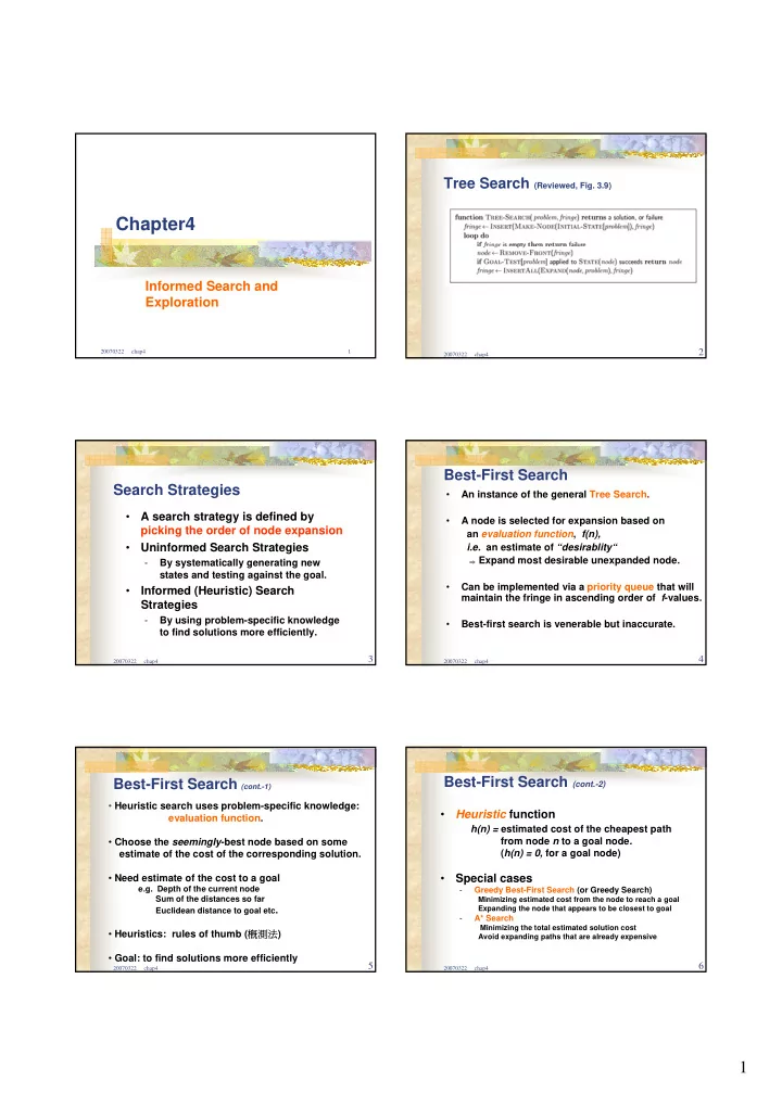
Tree Search (Reviewed, Fig. 3.9)

20070322 chap4

3

Search Strategies

A search strategy is defined by

picking the order of node expansion

Uninformed Search Strategies
By systematically generating new

states and testing against the goal.

Informed (Heuristic) Search

Strategies

By using problem-specific knowledge

to find solutions more efficiently.

20070322 chap4

4

An instance of the general Tree Search.
A node is selected for expansion based on

an evaluation function, f(n), i.e. an estimate of “desirablity“

⇒ Expand most desirable unexpanded node.

Can be implemented via a priority queue that will

maintain the fringe in ascending order of f-values.

Best-first search is venerable but inaccurate.

Best-First Search

20070322 chap4

5

Best-First Search (cont.-1)

Heuristic search uses problem-specific knowledge:

evaluation function.

Choose the seemingly-best node based on some

estimate of the cost of the corresponding solution.

Need estimate of the cost to a goal

e.g. Depth of the current node Sum of the distances so far Euclidean distance to goal etc.

Heuristics: rules of thumb (概測法)
Goal: to find solutions more efficiently

20070322 chap4

6

Heuristic function

h(n) = estimated cost of the cheapest path from node n to a goal node. (h(n) = 0, for a goal node)

Special cases
Greedy Best-First Search (or Greedy Search)

Minimizing estimated cost from the node to reach a goal Expanding the node that appears to be closest to goal

A* Search

Minimizing the total estimated solution cost Avoid expanding paths that are already expensive

Best-First Search (cont.-2)

SLIDE 2

2

20070322 chap4

7

Heuristics

Heuristic is derived from heuriskein in Greek,

meaning “to find” or “to discover”

The term heuristics is often used to describe

rules of thumb (經驗法則) or advice that are generally effective, but are not guaranteed to work in every case.

In the context of search, a heuristic is a function that

takes a state as an argument and returns a number that is an estimate of the merit of the state with respect to the goal.

20070322 chap4

8

Heuristics (cont.)

A heuristic algorithm

improves the average-case performance, does not necessarily improve the worst-case performance.

Not all heuristic functions are beneficial.
The time spent evaluating the heuristic function in order to

select a node for expansion must be recovered by a corresponding reduction in the size of the search space explored.

Useful heuristics should be computationally inexpensive!

20070322 chap4

9

Romania with step costs in km

Straight-line distances to Bucharest

20070322 chap4

10

Greedy Best-First Search

Heuristic function:

h(n) = estimated best cost to goal from n h(n) = 0 if n is a goal e.g. hSLD(n) = straight-line distance for route-finding

Function GREEDY-SEARCH(problem) return a solution or failure return BEST-FIRST-SEARCH(problem, h)

20070322 chap4

11

Greedy Best-First Search Example

Assume that we want to use greedy search

to solve the problem of travelling from Arad to Bucharest.

The initial state=Arad

20070322 chap4

12

Greedy Best-First Search Example (cont.-1)

The first expansion step produces:

Sibiu, Timisoara and Zerind

Greedy best-first will select Sibiu

SLIDE 3

3

20070322 chap4

13

Greedy Best-First Search Example (cont.-2)

If Sibiu is expanded we get:

Arad, Fagaras, Oradea and Rimnicu Vilcea

Greedy best-first search will select: Fagaras

20070322 chap4

14

Greedy Best-First Search Example (cont.-3)

If Fagaras is expanded we get:

Sibiu and Bucharest

Goal reached !!
Yet not optimal (see Arad → Sibiu → Rimnicu Vilcea → Pitesti)

20070322 chap4

15

Analysis of Greedy Search

Complete??

No (start down an infinite path and never return to try other possibilities)

(e.g. from Iasi to Fagaras)

Susceptible to false starts

Iasi → Neamt (dead end)

No Repeated states Checking

Iasi → Neamt → Iasi → Neamt → Iasi → ….. (oscillation)

Time?? (like depth-first search)

worst: O(bm), but a good heuristic can give dramatic improvement

m: the maximum depth of the search space

Space?? O(bm): keep all nodes in memory

20070322 chap4

16

Analysis of Greedy Search (cont.)

Optimal?? No (same as depth-first search)

(e.g. from Arad to Bucharest) Arad → Sibiu → Fagaras → Bucharest (450=140+99+211, is not shortest) Arad → Sibiu → Rim → Pitesti → Bucharest (418=140+80+97+101)

20070322 chap4

17

A* Search

To minimizing the total estimated solution cost
Evaluation function:

f(n) = estimated cost of the cheapest solution through n to goal = g(n) + h(n) g(n) = cost so far to reach n h(n) = estimated cost from n to the goal function A*-SEARCH(problem) returns a solution or failure return BEST-FIRST-SEARCH(problem, g+h)

20070322 chap4

18

Admissible Heuristic

A* search uses an admissible heuristic

i.e. h(n) ≤ h*(n)

where h*(n) is the true cost from n (Also h(n) ≥ 0 , so h(G) = 0 for any goal G)

Theorem:

If h(n) is admissible, A* using tree-search is optimal.

It is both complete and optimal if h never
verestimates the cost to the goal.

SLIDE 4

4

20070322 chap4

19

A* Search Example

Find Bucharest starting at Arad

f(Arad) = c(??,Arad)+h(Arad)=0+366=366

20070322 chap4

20

A* Search Example (cont.-1)

Expand Arrad and determine f(n) for each node

f(Sibiu)=c(Arad,Sibiu)+h(Sibiu)=140+253=393 f(Timisoara)=c(Arad,Timisoara)+h(Timisoara)=118+329=447 f(Zerind)=c(Arad,Zerind)+h(Zerind)=75+374=449

Best choice is Sibiu

20070322 chap4

21

A* Search Example (cont.-2)

Expand Sibiu and determine f(n) for each node

f(Arad)=c(Sibiu,Arad)+h(Arad)=280+366=646 f(Fagaras)=c(Sibiu,Fagaras)+h(Fagaras)=239+179=415 f(Oradea)=c(Sibiu,Oradea)+h(Oradea)=291+380=671 f(Rimnicu Vilcea)=c(Sibiu,Rimnicu Vilcea)+h(Rimnicu Vilcea) =220+192=413

Best choice is Rimnicu Vilcea

20070322 chap4

22

A* Search Example (cont.-3)

Expand Rimnicu Vilcea and determine f(n) for each node

f(Craiova)=c(Rimnicu Vilcea, Craiova)+h(Craiova)=360+160=526 f(Pitesti)=c(Rimnicu Vilcea, Pitesti)+h(Pitesti)=317+100=417 f(Sibiu)=c(Rimnicu Vilcea,Sibiu)+h(Sibiu)=300+253=553

Best choice is Fagaras

20070322 chap4

23

A* Search Example (cont.-4)

Expand Fagaras and determine f(n) for each node

f(Sibiu)=c(Fagaras, Sibiu)+h(Sibiu)=338+253=591 f(Bucharest)=c(Fagaras,Bucharest)+h(Bucharest)=450+0 =450

Best choice is Pitesti

20070322 chap4

24

A* Search Example (cont.-5)

Expand Pitesti and determine f(n) for each node

f(Bucharest)=c(Pitesti,Bucharest)+h(Bucharest)=418+0=418

Best choice is Bucharest
Optimal solution (only if h(n) is admissable)
Note values along optimal path

SLIDE 5

5

20070322 chap4

25

Optimality of A*

Suppose some suboptimal goal G2 has been generated and is in the queue. Let n be an unexpanded node on a shortest path to an optimal goal G.

20070322 chap4

26

Optimality of A* (cont.-1)

C* : cost of the optimal solution path

A* may expand some nodes before selecting a goal node.

Assume: G is an optimal and G2 is a suboptimal goal .

f(G2) = g(G2) + h(G2) = g(G2) > C* -------- (1) For some n on an optimal path to G, if h is admissible, then f(n) = g(n) + h(n) ≤ C*

------- (2)

From (1) and (2), we have f(n) ≤ C* < f(G2) So, A* will never select G2 for expansion.

20070322 chap4

27

Optimality of A*

(cont.-2)

BUT … graph search (instead of tree-search)
Discards new paths to repeated state.
Previous proof breaks down
Solution:
Add extra bookkeeping

i.e. remove more expensive of two paths.

Ensure that optimal path to any repeated state is

always first followed. Extra requirement on h(n): consistency (monotonicity)

20070322 chap4

28

Monotonicity (Consistency) of Heuristic

A heuristic is consistent if

h(n) ≤ c(n, a, n’) + h(n’) The estimated cost of reaching the goal from n is no greater than the step cost of getting to successor n’ plus the estimated cost of reaching the goal from n’

If h is consistent, we have

f(n’) = g(n’) + h(n’) = g(n) + c(n, a, n’) + h(n’) ≥ g(n) + h(n) = f(n) ⇒ f(n’) ≥ f(n) i.e. f(n) is non-decreasing along any path.

Theorem:

If h(n) is cosisient, A* using graph search is optimal.

20070322 chap4

29

Optimality of A* (cont.-3)

A* expands nodes in order of increasing f value

Gradually adds “f-contours” of nodes Contour i has all nodes with f = fi, where fi < fi+1

All nodes with f(n) > C* (optimal solution) are pruned.

20070322 chap4

30

Analysis of A* Search

Complete?? Yes

unless there are indefinitely many nodes with f ≤ f(G)

Space?? O(bd), keep all nodes in memory Optimal?? Yes, if the heuristic is admissible Optimally Efficient?? Yes

i.e. No other optimal algorithm is guaranteed to expand fewer nodes than A*

A* is not practical for many large-scale problems.

(Since A* usually runs out of space long before it runs out of time.)

SLIDE 6

6

20070322 chap4

31 Overcome the space problem of A*, without sacrificing

ptimality or completeness
IDA* (Iterative Deepening A*)
a logical extension of iterative deepening search to use

heuristic

the cutoff used is the f-cost (g+h) rather than the depth
RBFS (Recursive best-first search)
MA* (Memory-bounded A*)
SMA* (Simplified MA*)
is similar to A*, but restricts the queue size to fit into the

available memory

drop the worst-leaf node when memory is full

Memory Bounded Heuristic Search

20070322 chap4

32

RBFS (Recursive Best-First Search)

20070322 chap4

33

RBFS Example

140 118 75 =140+253 =118+329 =75+374 140 99 151 80 =(140+140)+366 =(140+80) +193 =(140+99) +176

Path until Rumnicu Vilcea is already expanded
Above node; f-limit for every recursive call is shown on top.
Below node: f(n)
The path is followed until Pitesti which has a f-value worse

than the f-limit.

20070322 chap4

34

RBFS Example (cont.-1)

Unwind recursion and store best f-value for current best leaf Pitesti

result, f [best] ← RBFS(problem, best, min(f_limit, alternative))

best is now Fagaras. Call RBFS for new best

best value is now 450

20070322 chap4

35

RBFS Example (cont.-2)

Unwind recursion and store best f-value for current best leaf Fagaras

result, f [best] ← RBFS(problem, best, min(f_limit, alternative))

best is now Rimnicu Viclea (again). Call RBFS for new best .

Subtree is again expanded. Best alternative subtree is now through Timisoara

Solution is found since because 447 > 417.

20070322 chap4

36

Analysis of RBFS

Complete?? Yes Time?? Exponential Space?? O(bd) Optimal?? Yes, if the heuristic is admissible IDA* and RBFS suffer from too little memory.

IDA* retains only one single number (the current f-cost limit)

RBFS is a bit more efficient than IDA*

Still excessive node generation

SLIDE 7

7

20070322 chap4

37 e.g. for the 8-puzzle branching factor: 3 depth: 22 # of states: 322 = 3.1 * 1010 9! /2= 181,440 (reachable distinct states) for the 15-puzzle # of states: ≅ 1013 How to find a good heuristic function ?

Heuristic Functions

20070322 chap4

38

Heuristic Functions (cont.)

Two commonly-used candidates

h1(n) = number of misplaced tiles =8 h2(n) = total Manhattan distance

(i.e. no. of squares from desired location to each tile)

= 3+1+2+2+2+3+3+2= 18

20070322 chap4

39

Effect of Heuristic Accuracy on Performance

h2 dominates (is more informed than) h1

If h2(n) >= h1(n) for all n (both admissible)

then h2 dominates h1 and is better for search

1200 random problems with solution lengths

from 2 to 24.

20070322 chap4

40

Heuristic Quality

Effective branching factor b* is defined by

A well-designed heuristic would have a value of b* close to 1, allowing fairly large problems to be solved.

A heuristic function h2 is said to be more informed

than h1 (or h2 dominates h1 ) if both are admissible and

A* using h2 will never expand more nodes than A*

using h1

d

b b b N ) ( ) ( 1 1

* 2 * *

+ + + + = + L ) ( ) ( ,

1 2

n h n h n ≥ ∀

20070322 chap4

41

Relaxed problems

A problem with fewer restrictions on the actions The cost of an optimal solution to a relaxed problem is an admissible heuristic for the original problem.

ABSolver

is a program that can generate heuristics automatically from problem definitions, using the “relaxed problem” method and various other techniques. generated a new heuristic for 8-puzzle better than preexisting heuristic found the first useful heuristic for Rubik’s cube puzzle.

Inventing Admissible Heuristics

20070322 chap4

42

Inventing Admissible Heuristics (cont.-1)

e.g. A tile can move from square A to square B if

A is horizontally or vertically adjacent to B and B is blank.

(P if R and S)

3 Relaxed problems:

(a) A tile can move from square A to square B if A is horizontally or vertically adjacent to B.

(P if R) --- derive h2

(b) A tile can move from square A to square B if B is blank.

(P if S)

(c) A tile can move from square A to square B.

(P) --- derive h1

SLIDE 8

8

20070322 chap4

43

Inventing Admissible Heuristics (cont.-2)

Composite heuristics

Given h1, h2, h3, … , hm ; none dominates any others. h(n) = max{h1 (n), h2 (n), … , hm (n)}

Subproblem

The cost of the optimal solution of the subproblem is a lower bound on the cost of the complete problem.

(To get tiles 1,2,3 and 4 into their correct positions, without worrying about what happens to the other titles.)

Pattern databases store the exact solution to for every possible

subproblem instance.

The complete heuristic is constructed using the patterns in the DB

20070322 chap4

44

Inventing Admissible Heuristics (cont.-3)

Weighted evaluation function :
Through learning from experience

Experience = solving lots of 8-puzzles An inductive learning algorithm can be used to predict costs for other states that arise during search.

Search cost

Good heuristics should be efficiently computable. ) ( ) ( ) 1 ( ) ( n wh n g w n fw + − =

20070322 chap4

45

Local Search and Optimization

Previously: systematic exploration of search

space.

Path to goal is solution to problem
YET, for some problems path is irrelevant.

e.g 8-queens What quantities of quarters, nickels, and dimes add up to $17.45 and minimizes the total number of coins

Different algorithms can be used
Local search

20070322 chap4

46

Local Search Algorithms

Local search does not keep track of

previous solutions

Using a single current state (rather than

multiple paths) and move only to neighboring states

Advantages
Use a small amount of memory (usually

constant amount)

Often find reasonable (note we aren’t saying
ptimal) solutions in infinite search spaces

20070322 chap4

47

To find the best state according to

an Objective Function Example

f (q, d, n) = 1,000,000, if q*0.25 + d*0.1 + n*0.05 != 17.45 = q + n + d, otherwise To minimize f

Optimization Problems

20070322 chap4

48

Looking for global maximum (or minimum)

SLIDE 9

9

20070322 chap4

49

Hill-Climbing Search

Like climbing Everest in thick fog with amnesia

20070322 chap4

50

Hill-Climbing Search (cont.-1)

Only record the state and it evaluation instead
f maintaining a search tree
“is a loop that continuously moves in the

direction of increasing value”

It terminates when a peak is reached.
Hill climbing does not look ahead of the

immediate neighbors of the current state.

Hill-climbing chooses randomly among the set
f best successors, if there is more than one.
Hill-climbing i.e. greedy local search

20070322 chap4

51

Hill-climbing example

a) shows a state of h=17 and the h-value for each possible

successor. (h=3+4+2+3+2+2+1)

b) A local minimum in the 8-queens state space (h=1).

a) b)

20070322 chap4

52

Hill-Climbing Search (cont.-2)

Problems:

Local Maxima: search halts prematurely
Plateaux: search conducts a random walk
Ridges: search oscillates with slow progress

Creating a sequence of local maximum that are not directly connected to each other. From each local maximum, all the available actions point downhill.

20070322 chap4

53

Hill-climbing variations

Stochastic hill-climbing

Random selection among the uphill moves. The selection probability can vary with the steepness of the uphill move.

First-choice hill-climbing

Like stochastic hill climbing but by generating successors randomly until a better one is found.

Random-restart hill-climbing

Tries to avoid getting stuck in local maxima.

20070322 chap4

54

Simulated Annealing

SLIDE 10

10

20070322 chap4

55

Simulated Annealing (cont.-1)

Idea: escape local maxima by allowing some "bad"

moves but gradually decrease their frequency

A term borrowed from metalworking
We want metal molecules to find a stable location

relative to neighbors

heating causes metal molecules to move around and to

take on undesirable locations

during cooling, molecules reduce their movement and

settle into a more stable position

annealing is process of heating metal and letting it cool

slowly to lock in the stable locations of the molecules

20070322 chap4

56

Simulated Annealing (cont.-2)

Select a random move at each iteration
Move to the selected node if it is better than

the current node.

The probability of moving to a worse node

decreases exponentially with the ``badness'' of the move, i.e.

The temperature T changes according to a

schedule.

T E

e

/ Δ

20070322 chap4

57

Simulated Annealing (cont.-3)

One can prove: If T decreases slowly enough,

then simulated annealing search will find a global

ptimum with probability approaching 1
Widely used in VLSI layout, airline scheduling, etc

20070322 chap4

58

Local Beam Search

Keep track of k states rather than just one
Start with k randomly generated states
At each iteration, all the successors of all k

states are generated

If any one is a goal state, stop; else select the k

best successors from the complete list and repeat.

20070322 chap4

59

Genetic algorithms

A successor state is generated by combining two

parent states

Start with k randomly generated states (population

)

A state is represented as a string over a finite alphabet

(often a string of 0s and 1s)

Evaluation function (fitness function).

Higher values for better states.

Produce the next generation of states by selection,

crossover, and mutation

20070322 chap4

60

Genetic Algorithms (cont.-1)

Fitness function: number of non-attacking pairs of

queens (min = 0, max = 8 × 7/2 = 28)

24/(24+23+20+11) = 31%
23/(24+23+20+11) = 29% etc