SLIDE 1
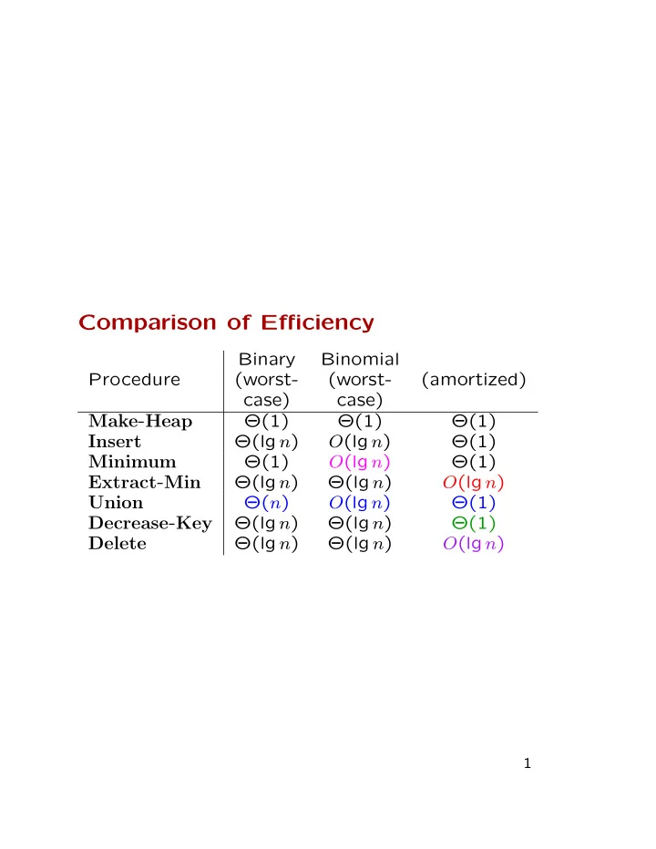
Comparison of Efficiency
Binary Binomial Procedure (worst- (worst- (amortized) case) case)
Make-Heap
Θ(1) Θ(1) Θ(1)
Insert
Θ(lg n) O(lg n) Θ(1)
Minimum
Θ(1) O(lg n) Θ(1)
Extract-Min
Θ(lg n) Θ(lg n) O(lg n)
Union
Θ(n) O(lg n) Θ(1)
Decrease-Key
Θ(lg n) Θ(lg n) Θ(1)
Delete
Θ(lg n) Θ(lg n) O(lg n)
1
SLIDE 2 Chapter 23: Minimum Spanning Tree Let G = (V, E) be a connected (undirected)
- graph. A spanning tree of G is a tree T that
consists of edges of G and connects every pair of nodes. Let w be an integer edge-weight function. A minimum-weight spanning-tree is a tree whose weight weight respect to w is the smallest of all spanning trees of G.
2
SLIDE 3
a i c f e g h
4 8 7 6 2 8 9 10 4 7 1 2 14 11
b d
3
SLIDE 4
Safe edges and cuts A : expandable to an MST e ∈ E − A is safe for A if A ∪ {e} : expandable to an MST or an MST already a cut of G : a partition (S, V − S) of V an edge e crosses (S, V − S) if e connects a node in S and one in V − S (S, V − S) respects A ⊆ E if no edges in A cross the cut
b e h
4 8 6 2 8 9 10 4 7 1 2 14 11 7
S V-S a i c f d g
For any edge property Q, a light edge w.r.t. Q is one with the smallest weight among those with the property Q
4
SLIDE 5 Theorem A Let G = (V, E) be a connected (undirected) graph with edge-weight function
- w. Let A be a set expandable to an MST, let
(S, V − S) be a cut respecting A, and let e = (u, v) be a light edge crossing the cut. Then e is safe for A. Proof Let T be an MST containing A and not containing e. There is a unique path ρ in T from u to v. ρ has an edge crossing (S, V − S). Pick one such edge d. Then T ′ = T ∪ {e} − {d} is a spanning tree such that w(T ′) = w(T) so T ′ is an MST and e is safe. Corollary B Every light edge connecting two distinct components in GA = (V, A) is safe for A.
5
SLIDE 6 Kruskal’s Algorithm Maintain a collection of connected components and construct an MST A. Initially, each node is a connected component and A = ∅. Examine all the edges in the nondecreasing
- rder of weights.
- If the current edge connects two different
components, add e to A to unite the two components. The added edge is a light edge; otherwise, an edge with smaller weight should have already united the two components.
6
SLIDE 7
4 8 7 9 10 14 4 2 1 6 2 7 11 4 8 7 9 10 14 4 2 1 6 7 11 2 4 8 7 9 10 14 4 2 1 6 7 11 2 4 8 7 9 10 14 4 2 1 6 7 11 2 4 8 7 9 10 14 4 2 1 6 7 11 2 4 8 7 9 10 14 4 2 1 6 7 11 2 4 8 7 9 10 14 4 2 1 6 7 11 2 4 8 7 9 10 14 4 2 1 6 7 11 2 8 8 8 8 8 8 8 8
7
SLIDE 8
4 8 7 9 10 14 4 2 1 6 7 11 2 4 8 7 9 10 14 4 2 1 6 7 11 2 4 8 7 9 10 14 4 2 1 6 7 11 2 4 8 7 9 10 14 4 2 1 6 7 11 2 4 8 7 9 10 14 4 2 1 6 7 11 2 4 8 7 9 10 14 4 2 1 6 7 11 2 8 8 8 8 8 8
8
SLIDE 9
Implementation with “disjoint-sets” 1 A ← ∅ 2 for each vertex v ∈ V do 3
Make-Set(v)
4 reorder the edges so their weights are in nondecreasing order 5 for each edge (u, v) ∈ E in the order do 6 if Find-Set(u) = Find-Set(v) then 7 A ← A ∪ {(u, v)} 8
Union(u, v)
9 return A
9
SLIDE 10
The number of disjoint-set operations that are executed is 2E + 2V − 1 = O(E), out of which V are Make-Set operations. What is the total running time?
10
SLIDE 11
The total cost of the disjoint-set operation is O(E lg∗ V ) if the union-by-rank and the path-compression heuristics are used. Sorting the edges requires O(E log E) steps. We can assume E ≥ V − 1 and E ≤ V 2. So, it’s O(E log V ) steps.
11
SLIDE 12 Prim’s algorithm Maintain a set of edges A and a set of nodes
- B. Pick any node r as the root and set B to
{r}. Set A to ∅. Then repeat the following V − 1 times:
- Find a light edge e = (u, v) connecting
u ∈ B and v ∈ V − B.
12
SLIDE 13
4 8 7 9 10 14 4 12 21 6 2 7 11 4 8 7 9 10 14 4 12 21 6 2 7 11 4 8 7 9 10 14 4 12 21 6 2 7 11 4 8 7 9 10 14 4 12 21 6 2 7 11 4 8 7 9 10 14 4 6 2 7 11 4 8 7 9 10 14 4 6 2 7 11 4 8 7 9 10 14 4 6 2 7 11 4 8 7 9 10 14 4 6 2 7 11 4 8 7 9 10 14 4 6 2 7 11 8 8 8 8 8 8 8 8 8 21 21 21 21 21 12 12 12 12 12
13
SLIDE 14
Implementation Using a Priority Queue For each node in Q, let key[v] be the minimum edge weight connecting v to a node in B. By convention, key[v] = ∞ if there is no such edge. For each node v record the parent in the field π[v]. This is the node u such that (u, v) is the light edge when v is added to B. An implicit definition of A is {(v, π[v]) | v ∈ V − {r} − Q}.
14
SLIDE 15
1 Q ← V 2 for each u ∈ Q do key[u] ← ∞ 3
key[r] ← 0
4 π[r] ← nil 5 while Q = ∅ do 6 u ← Extract-Min(Q) 7 for each v ∈ Adj[u] do 8 if v ∈ Q and w(u, v) < key[v] then 9 π[v] ← u 10
key[v] ← w(u, v)
Line 3 forces to select r first. Lines 7-10 are for updating the keys. Implement Q using a heap. The running time is V · (the cost of Build-Heap) + (V − 1) · (the cost of Extract-Min) + E · (the cost of Decrease-Key).
15
SLIDE 16
If either a binary heap or a binomial heap is used, the running time is: V · O(1) + (V − 1) · O(lg V ) + E · O(lg V ) = O((E + V ) lg V ) = O(E lg E), which is the same as the running time of Kruskal’s algorithm. If a Fibonacci heap is used, the running time is: V · O(1) + (V − 1) · O(lg V ) + E · O(1) = O(V lg V + E), which is better than the running time of Kruskal’s algorithm.
16