Completeness of Resolution using Tableaux A2ai Example . Given: - - PowerPoint PPT Presentation

AUTOMATED REASONING SLIDES 9 to 11 (Appendix A2): RELATIONS between RESOLUTION and TABLEAU Completeness of Resolution via tableaux A useful notation (chain notation) Relation of ME with linear resolution The UNIFY - AT - END tableau development Parallel Model Elimination

KB-AR - 09 A2ai

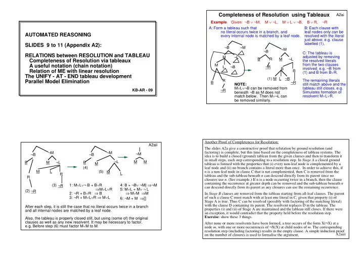
• Example. Given: ¬B ∨ ¬M, M ∨ ¬L, M ∨ L ∨ ¬B, B ∨ R, ¬R

A: Form a tableau such that no literal occurs twice in a branch, and every internal node is matched by a leaf node. B: Each clause with leaf nodes only can be resolved with the literal just above. e.g. clause labelled (1). ¬B ¬M B R M ¬L ¬R B R M L ¬B ¬R (1) C: The tableau is adjusted by removing the resolved literals from the two clauses

• involved. e.g. ¬B from

(1) and B from B∨R. The remaining literals still match above and the tableau still closes. e.g. Simulates formation of resolvent M∨L∨R. NOTE: M∨L∨¬B can be removed from beneath ¬B as M does not match below. Then M∨¬L can be removed similarly. ¬B ¬M M ¬L M L ¬B B R ¬R

Completeness of Resolution using Tableaux

A2aii ¬B ¬M B M M (4) ¬L L (5) ¬M M M 1: M∨L∨¬ B + B∨R ⇒M∨L∨R 2: ¬R + B∨R ⇒ B 3: ¬R + M∨L∨R ⇒ M∨L 4: B + ¬B∨ ¬M} ⇒¬M 5: M∨L + M∨ ¬ L ⇒ M∨M ⇒M 6: ¬M + M ⇒[] After each step, it is still the case that no literal occurs twice in a branch and all internal nodes are matched by a leaf node. Also, the tableau is properly closed still, but using (some of) the original clauses as well as any new resolvent. It may be necessary to factor. e.g. Before step (6) must factor M∨M to M. ¬B ¬M B M ¬L R ¬R M L (3) R ¬R (2) A2aiii Another Proof of Completeness for Resolution: The slides A2a give a constructive proof that refutation by ground resolution (and factoring) is complete, but this time based on the completeness of tableau systems. The idea is to build a closed (ground) tableau from the given clauses and then to transform it in small steps, each step corresponding to a resolution step. In Stage A a closed ground tableau is formed with the properties that (i) every non-leaf node is complemented by a leaf node and (ii) no branch contains a literal more than once. In order to achieve this, if n is a non-leaf node in clause C that is not complemented, then C is removed from the tableau and the sub-tableau beneath n can descend directly from its parent since no closures use n. (See example.) If n is a node occurring twice in a branch, then the clause containing the occurrence at greater depth can be removed and the sub-tableau beneath n can descend directly from its parent as any closures can use the remaining occurrence. In Stage B clauses are removed from the tableau starting from all-leaf clauses. The parent

• f such a clause C must match with at least one literal in C, given that property (i) of

Stage A is true. Thus C can be resolved (possibly with factoring of the matching literal) with the clause D containing its parent. The resolvent replaces D in the tableau. The properties (i) and (ii) of Stage A are maintained and the tableau still closes. If there were an exception, it would contradict that the property held before the resolution step. Exercise: show these 3 things. After none or more resolvents have been formed, a tree occurs of the form X(¬X) at a node m, with one or more occurrences of ¬X(X) at child nodes of m. The corresponding resolution step (including factoring) results in the empty clause. A simple induction proof

• n the number of closures is used to formalise the argument.

A2bi Relation between ME tableau and Linear resolution refinements (1) ME-tableaux are closely related to the linear refinement of resolution. This refinement is

• utlined below. It was introduced before free-variable ME-tableaux, as were the various

restrictions of the refinement. However, there is one particular restriction, called SL- resolution, which corresponds exactly to free-variable ME-tableau. When the generalised closure rule is included, then more general linear resolution proofs can be simulated by

• tableaux. The relationship between the two systems is detailed further in the chapter notes
• n clausal tableaux, if you're interested.

Strategy of Linear resolution First select an initial clause called top in the set of support of set of clauses S: The set of support of S = {C |C ∈S & S-{C} is satisfiable}; i.e. each C in the set of support is necessary to derive [ ]. Next resolve C with an input clause from S (possibly a second copy of top). Then, at each subsequent step resolve the latest resolvent with either an input clause, or a previous resolvent (called ancestor resolution). e.g. If the refutation is R0 , R1 , R2 , ...., [ ], where R0 is the top clause, then R2 is formed by resolving R1 with an input clause or with R0 or with R1. Linear resolution appears to be quite natural as it generalises top-down/goal-directed

• reasoning. The search space is a tree, each branch being one possible linear derivation, so

efficient search methods and Prolog technology can be employed. The example shown on the right in A2bv looks as follows: Px ∨Q, Rx ∨Q, ¬Rb ∨Q, Q∨Q (i.e. Q), [ ].The ancestor resolution step is between ¬Rb ∨Q and Rx ∨Q, deriving Q∨Q, which factors to Q. A2bii Relation between ME tableau and Linear resolution refinements (2) Next we explain how a ME-tableau relates to a linear resolution derivation. The idea is that at each ME-step the disjunction of the leaf literals in open branches is the latest resolvent of the corresponding linear refutation. In the example on A2bv, after the first closure the leaf literals

• f the open branches are Rx and Q, which are exactly the literals in the second resolvent in the

derivation, as given in A2bi. Similarly, after the second closure the leaf literals are ¬Rb and Q, exactly the third clause in the derivation. The various tableau steps correspond as follows: i) Extension corresponds to resolution of an input clause with the latest resolvent, ie one that has been extended in the branch before, choosing to resolve on a literal most recently introduced into the resolvent. ii) Closure corresponds to resolution of the latest resolvent with an ancestor resolvent, but in a quite restricted way. If the previous resolvent used was R = L ∨ C, where L was the literal resolved upon in R before, then R can only be used again by resolving on L. Moreover, the same "instance" of R must be used. That means that both copies of R must use the same instantiation, i.e. it is R used twice, not R and a copy of R. This is sufficient to ensure that the 2 occurrences of clause C in the resolvent that arise from the two steps using R will factor. In fact, as long as this latter property holds, the other restriction can be relaxed; this would correspond to using the generalised closure rule. In a normal ME tableau, the restriction on closure is automatically ensured by the structure of the tableau, since only one instance of each literal occurrence is allowed. On A2bv, notice that in order to use Rx a second time with substitution b, it is necessary to use a second occurrence, which brings with it a second occurrence of Q. The same effect can be obtained by allowing a second instance of Rx (namely when x==b), as in the generalised closure rule of ME. As an example, A2biii/A2biv shows the linear refutation corresponding to the LH tableau of 11bi. A2biii Model Elimination Tableau Simulation of Linear Resolution Consider the tableau shown on 11bi (repeated on A2biv) and the corresponding linear resolution derivation, which is also shown. The top clause of the linear derivation is Fx1∨Hx1, which is the first clause in the ME tableau. The first two steps resolve with input clauses and the resolvents of each step correspond to the leaf literals of the open branches of the tableau. Notice that the third step, which resolves with Fx1 for a second time and which derives Hb ∨Hb, is an ancestor matching step in the tableau and that there is only one instance of Fx1, which is the one enforced by the unifier of this step. The two occurrences of Hb appear just once in the tableau. In the resolution proof the resolution is between the clause ¬Fb ∨Hx1 and a copy of the ancestor Fx1∨Hx1, say Fx3∨Hx3, which yield Hb ∨Hx1. This factors to Hb and corresponds with the tableau version. The restricted linear resolution strategy, which simulates ME, only allows resolution with the ancestor instance Fx1∨Hx1, not a fresh copy of Fx ∨Hx. It also restricts to using Fx1, the literal prevously resolved upon. If that instance were to be used later in the derivation, it is only the instance Fb ∨Hb that may be used. The unrestricted liner resolution strategy will also allow ¬Fx2 to resolve with a fresh copy of the ancestor Fx ∨Hx. In the tableau, the ancestor matching step (corresponding to using the copy) is not available because Fx1 from Fx1∨Hx1 is not part of the "history" leading to ¬Fx2. That is why ancestor use is restricted to using the literal previously resolved upon. The generalised closure rule corresponds to using the copy to resolve with the current resolvent R, as long as the copy of the remaining literals safely factors with the literals in R. In general linear resolution the step of ancestor resolution is even more flexible - any literal in the ancestor can be used, not just the literal that was used the first time the ancestor was involved in a resolution step. More on this is in the `Chapter' notes if you're interested. Fx1∨Hx1 ¬Fx ∨Gx} {Gx1∨Hx ¬Gx ∨ ¬Fb} ¬Fb ∨Hx1 Hb ∨Hb Hb ⇓ ¬Hb ∨ ¬Fx ¬Fx2 Fx ∨Hx Hx2 ¬Ha x1==b (x2==a) [ ] A2biv Comparison of Linear resolution and ME for the clauses: ¬Ha , ¬Gx ∨ ¬Fb , ¬Fx ∨ ¬Hb , Gx ∨ ¬Fx, Fx ∨ Hx ¬F(x2) x2==x1 Fx1 Hx1 ⇒ Hb G(x2) ⇒Gx1 ¬Hb ¬ Fx2 ¬Gx1 Fx2 Hx2 ¬Fb x1==b ¬Ha x2==a See A2biii for commentary on these derivations

A2bv Generalised closure rule of ME can simulate Linear Resolution Rx ∨ ¬Px, Px ∨Q, ¬Ra ∨ ¬Rb, ¬Q A ME tableau can be seen as simulating a special kind of linear resolution strategy. In the derivation on the right the two copies of Q derived from the same parent literal will factor. This will always be the case in the tableau if variables in the branch closing by the generalised closure rule do not occur in any remaining leaf literals. A linear resolution strategy. Q Px ¬Px Rx ¬Ra x=a ¬Rb Px Q ¬Px ¬Q ¬Q =>Ra Rx Px ∨Q ¬Px ∨Rx Rx ∨Q ¬Ra ∨¬Rb Q ∨Q ¬Q ¬Rb ∨Q [ ] A2ci Chain Notation for ME Tableaux: For interest, slide A2cii shows a convenient representation for ME-tableaux, called the chain notation, which is possible because such tableaux are developed from left to right. This notation enables a complete search space to be represented in 2 dimensions. A ME-tableau is maintained as a chain of literals. There are two types of entry, boxed and un- boxed literals. The top clause forms the first chain with the leftmost literal the next to be selected and all literals unboxed. A chain may (i) be extended by a new clause, (ii) be extended by ancestor matching or (iii) be truncated, corresponding, respectively, to tableau extension, ancestor closure or moving to the next branch to develop. (i) results in the matched literal becoming boxed and literals in the (added) matching clause (not including the complementary literal) being appended to the left of the chain. (ii) results in the leftmost literal being boxed if it unifies with a boxed literal to its right. (iii) removes leftmost boxed literals. A chain represents the remaining open branches of the ME tableau formed so far, which can be re-constructed from the chain. Each unboxed literal is a leaf literal L of the tableau. Its ancestors, forming the rest of the branch, are all the boxed literals to its right (the first boxed literal to the right being the parent of L). Alternatively, all literals to the left of a boxed literal are its decendants. The example on A2cii illustrates. Regular tableaux can be enforced by not allowing a step that would result in an unboxed literal being duplicated by another boxed literal to its right. Also, if an unboxed literal is duplicated by an unboxed literal to its right, then the leftmost literal can be boxed, corresponding to the "merge" operation. A2cii ¬B∨ ¬M, M∨ ¬L, M∨L∨ ¬B, B∨R, ¬R top clause ¬B¬M extension R ¬B ¬M extension R ¬B ¬M truncation ¬M extension L¬B ¬M extension M L ¬B ¬M ancestor matching M L ¬B ¬M truncation ¬B ¬M extension R ¬B ¬M extension R ¬B ¬M truncation [] ¬B B R ¬R ¬M M L ¬B ¬L M B R ¬R Looping: If a literal occurs in a chain twice, the leftmost unboxed, the right

• ccurrence boxed, the leftmost indicates

a duplication.

CHAIN NOTATION - A handy shorthand

Merging: If a literal

• ccurs in a chain twice,

both times unboxed, the leftmost can be merged with the right copy. A2di How else could the free variable method be systematic? The ME approach is "unify as you go" What about "unify at the end"? How could tableau development be controlled? Possibilities for controlling Unify-at-the-end:

• Restrict total no. of clause instances over all branches / over each branch,
• r number of instances of each clause over all branches / over each branch.
• Likely to get many literals in a branch that cannot possibly unify; the

branches of which they are a part can be pruned. e.g.

• If only one occurrence of Hx in a branch then no need for two instances of

a clause containing ¬H(y), as they would have to be the same.

• If no copies of Hx in a branch then no use for ¬Hy.

Good/bad points of Unify-at-the-end:

• If not many quantifiers "unify at end" may be better.
• May only be one binding for a particular branch. Selecting it can restrict

unifiers in other branches.

• May be able to close branches without unifying. No backtracking (over

those branches).

• May have many unifiers in a branch; all have to be tried.

Comparison between Unify-at-the-end and Unify-as-you-go in ME tableaux

A2dii Constructing Free Variable Tableaux When constructing a free variable tableau, you may do it in one of two ways, which could be called "unify-as-you-go", or "unify-at-the-end". Slides 9-11 used the unify-as-you-go method and the alternative approach to closure is shown on Slides A2d: instead of closing each branch "as you go" and propagating the bindings across the whole tableau, it is noted when a branch can close and what the corresponding binding is, but no propagation takes place. The tableau on Slide A2diii is constructed using "unify-at-the-end". In the construction, if a branch can be closed by unifying two complementary literals, then it is marked as possibly

• closed. All possible unifiers that may lead to closure can be recorded as a label of the branch.

When every branch has such a potential closure, a single unifier must be constructed using one unifier from the label of each branch in the tableau. For the example on A2diii it results in the combined unifier (ie unify the individual unifiers) {x2==w1==g(n), x1==y1==x3==z1==n, u1==f(g(n)), y2==f(g(n))}. If it is not possible to construct a single unifier, then a different set

• f closures must be found (which may involve further extending the tableau) and another

combined unifier sought. This is in contrast to the "unify-as-you-go" kind of construction, illustrated on Slide 9ciii, where whenever a closure is made that requires a binding to be made to one or more free variables, the substitution is applied to all occurrences in the tableau of those newly bound variables. This guarantees consistency of the bindings as the tableau is constructed. Only one binding may be made to any free variable. The unify-as-you-go approach is useful for most applications, especially those using data structures, when it may be necessary for a piece of data to be used many times. If it is known (or quite possible that) each sub-sentence of each sentence is to be used only once or a very few times, the unify-at-the-end approach can be a reasonable one. (1) div(x,x), (2) less(1,n), (3) div(u,w) ∧ div(w,z) → div(u,z) (4) ¬(div(g(x),x) ∧ less(1,g(x)) ∧ less(g(x),x) ) → pr(x) (5) less(1,x)∧less(x,n)→div(f(x),x)∧pr(f(x)) Show ∃ ∃ ∃ ∃y (pr(y)∧ ∧ ∧ ∧div(y,n)) A2diii ¬∃y (pr(y)∧div(y,n)) ¬(pr(y1) ∧div(y1,n)) div(g(x1),x1) ∧ less(1,g(x1)) ∧ less(g(x1),x1) pr(x1) div(f(x2), x2) pr(f(x2)) ¬ (pr(y2)) ∧div(y2,n)) div(u1,z1) ¬ less(1,x2) ¬ less(x2,n) x2==g(x1) x2==g(x1) x1==n (or x2==1 is possible) ¬ div(u1,w1) ¬div(w1,z1) u1==f(x2) w1==x2 z1==x1 w1=g(x1) ¬ pr(y2) ¬ div(y2,n) y2==f(x2) ¬ pr(y1) ¬ div(y1,n) y1==x1 y1==n x3==n div(x3,x3) y2==u1, z1==n Gives: { x2==w1==g(n), x1==y1==x3==z1==n, u1==y2==f(g(n))} Free variable rules Unify at the end A2div E.g. Given: Fxa ∨Fg(x)x , Fxa ∨Fxg(x), ¬ Fxa ∨ ¬ Fxz ∨ ¬ Fzx Fx1a Fg(x1)x1 Fx2a Fx2g(x2) Fx3a Fx3g(x3) ¬Fx4a ¬Fx4z1 ¬Fz1x4 ¬Fx5a ¬Fx5z2 ¬Fz2x5 ¬Fx6a ¬Fx6z3 ¬Fz3x6 ¬Fx7a ¬Fx7z4 ¬Fz4x7 Assume at most one instance of each clause will be used in each branch. A successful unification is x4, z1, x1 all bound to a ; i.e. didn't need Fx2a ∨Fx2g(x2) in LH branch - it can be removed - so only need

• ne of the copies of

¬Fxa ∨ ¬Fxz ∨ ¬Fzx x6 bound to x3 and z3 and x3 bound to a; x7 bound to g(a), z4 bound to a.

• Sections of the tableau (indicated by

dotted lines) can be developed in parallel.

• If the tableau is ME style then

possibilities for re-use can be anticipated: eg if S occurs in closure below branch (ii) it can be closed in the same way as the closure below S in branch (i). Anticipate this by adding ¬S to branch (ii). 11ei

Parallel ME : Propositional case

• Each branch of a clausal tableau

can be distributed to a separate

• process. This is called and-

parallelism as every branch must close for a refutation.

• This is different from or-

parallelism in which each process is instead given a branch of the search space. eg in the tree on the left, if KLM (ie K∨L∨M) matched with more than one clause (as it does here: KLM matches with given clauses ¬KST and ¬K¬S), then there would be two branches of the search space. Process1 is given the search space using ¬KST and process2 the search space using ¬K¬S. If process2 finished before process1 then process1 can be terminated. K L M ¬K S T ¬S ¬K ¬S ¬K ¬K ¬L (ii) (i)

Parallel ME: First Order case

11eii

• In the and-parallel development to cope with potentially infinite tableau,

each section is developed to a fixed depth. Failure to find a proof causes the depth to be increased for a second attempt.

• Shared (ie non-universal) variables pose a problem:

e.g. Given: ¬Pxy ∨ ¬Pyx, Pf(u)u ∨ Pua, {Pvf(v) ∨ Pva Pf(u1)u1 Pu1a

• Values of u1 must be reconciled

between two processes.

• Pu1a can close with u1==a. It

can also close with u1==f(a). Are there any more values?

• Within a finite depth the number
• f values will be finite.
• Pf(u1)u1 can also close

(eventually) with u1 ==a.

• Each solution is passed up to

the parent process to be reconciled.

• Only bindings mentioned in

ancestor nodes are retained. ¬Px1y1 u1==x1 y1==a ¬Py1x1 u1==y1 x1==a Reconcile: obtain u1==x1==y1==a; Retain u1==a.

• If u1 were

universal, then can use a technique similar to the generalised closure rule. 11eiii Parallel Clausal Tableau Development: Slides 11e illustrate some possibilities for and-parallel execution within a clausal

• tableau. Each branch, called a section on 11ei, can be given to a separate processor.

It's possible to anticipate some possible cases for re-use as shown on the slide. The first order case is more complex as bindings must be preserved across branches for the shared (ie non-universal) free variables. One method is for each branch below a node n to be evaluated independently, finding as many bindings as possible for the variables occurring in the literal at n (to some max. depth to guarantee termination). The bindings are then reconciled (i.e. combined) at the node n with those from other sibling branches of n (i.e. only bindings which belong to the solution set of every sibling branch are retained, possibly further instantiated). Finally, only bindings to variables occurring in an ancestor of n need be kept for further propagation. E.g. let ground P occur at n's parent. Then n matches with P and let n's siblings be Q(x1) and R(x1). Although x1 must be reconciled with some binding, the particular binding is not relevant to the parent of n, unless x1 occurs elsewhere in the tableau. As this is not the case, the empty binding would be retained to pass back up the

• tableau. However, notice that the following circumstance could occur: x1 is bound

in another branchto some non-universal variable z in some ancestor of n, say x1==z, and also to x1==a, then the reconciled binding z==a is relevant, since z occurs in an ancestor of n. If all reconciliations fail, then no bindings are retained. A2ei

Summary of Slides 9 - 11 (Appendix 2)

• 1. Different unification regimes can be employed in ME tableau,

such as ``unify-as-you-go'', or ''unify-at-the-end''.

• 2. The completeness of resolution can be shown using tableaux. No

doubt, by controlling the style of tableau formed - e.g. ordering use

• f clauses in any branch – specific sorts of resolution proofs can be

derived.

• 3. ME tableau are related to linear resolution. The correspondence

imposes restrictions on the linear resolution, which is partially relaxed if the generalised closure rule is used.

• 4. A useful chain notation exists to represent tableau as a list of

boxed and unboxed literals.

• 5. With care ME tableaux can be evaluated in parallel.