CPU Scheduling The scheduling problem: - Have K jobs ready to run - - - PowerPoint PPT Presentation

CPU Scheduling

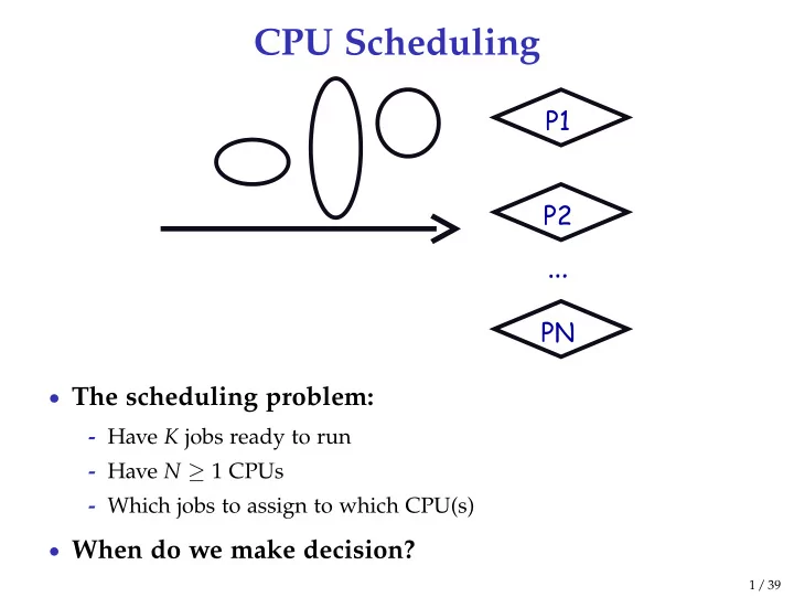
• The scheduling problem:
• Have K jobs ready to run
• Have N ≥ 1 CPUs
• Which jobs to assign to which CPU(s)
• When do we make decision?

1 / 39

CPU Scheduling

new ready waiting running terminated

I/O or event completion I/O or event wait scheduler dispatch interrupt exit admitted

• Scheduling decisions may take place when a process:
• 1. Switches from running to waiting state
• 2. Switches from running to ready state
• 3. Switches from new/waiting to ready
• 4. Exits
• Non-preemptive schedules use 1 & 4 only
• Preemptive schedulers run at all four points

2 / 39

Scheduling criteria

• Why do we care?
• What goals should we have for a scheduling algorithm?

3 / 39

Scheduling criteria

• Why do we care?
• What goals should we have for a scheduling algorithm?
• Throughput – # of procs that complete per unit time
• Higher is better
• Turnaround time – time for each proc to complete
• Lower is better
• Response time – time from request to first response

(e.g., key press to character echo, not launch to exit)

• Lower is better
• Above criteria are affected by secondary criteria
• CPU utilization – fraction of time CPU doing productive work
• Waiting time – time each proc waits in ready queue

3 / 39

Example: FCFS Scheduling

• Run jobs in order that they arrive
• Called “First-come first-served” (FCFS)
• E.g.., Say P1 needs 24 sec, while P2 and P3 need 3.
• Say P2, P3 arrived immediately after P1, get:
• Dirt simple to implement—how good is it?
• Throughput: 3 jobs / 30 sec = 0.1 jobs/sec
• Turnaround Time: P1 : 24, P2 : 27, P3 : 30
• Average TT: (24 + 27 + 30)/3 = 27
• Can we do better?

4 / 39

FCFS continued

• Suppose we scheduled P2, P3, then P1
• Would get:
• Throughput: 3 jobs / 30 sec = 0.1 jobs/sec
• Turnaround time: P1 : 30, P2 : 3, P3 : 6
• Average TT: (30 + 3 + 6)/3 = 13 – much less than 27
• Lesson: scheduling algorithm can reduce TT
• Minimizing waiting time can improve RT and TT
• What about throughput?

5 / 39

View CPU and I/O devices the same

• CPU is one of several devices needed by users’ jobs
• CPU runs compute jobs, Disk drive runs disk jobs, etc.
• With network, part of job may run on remote CPU
• Scheduling 1-CPU system with n I/O devices like

scheduling asymmetric (n + 1)-CPU multiprocessor

• Result: all I/O devices + CPU busy =

⇒ n+1 fold speedup!

grep matrix multiply running waiting for disk waiting in ready queue

• Overlap them just right? throughput will be almost doubled

6 / 39

Bursts of computation & I/O

• Jobs contain I/O and computation
• Bursts of computation
• Then must wait for I/O
• To Maximize throughput
• Must maximize CPU utilization
• Also maximize I/O device utilization
• How to do?
• Overlap I/O & computation from

multiple jobs

• Means response time very important

for I/O-intensive jobs: I/O device will be idle until job gets small amount of CPU to issue next I/O request

7 / 39

Histogram of CPU-burst times

• What does this mean for FCFS?

8 / 39

FCFS Convoy effect

• CPU-bound jobs will hold CPU until exit or I/O

(but I/O rare for CPU-bound thread)

• long periods where no I/O requests issued, and CPU held
• Result: poor I/O device utilization
• Example: one CPU-bound job, many I/O bound
• CPU-bound job runs (I/O devices idle)
• CPU-bound job blocks
• I/O-bound job(s) run, quickly block on I/O
• CPU-bound job runs again
• I/O completes
• CPU-bound job continues while I/O devices idle
• Simple hack: run process whose I/O completed?
• What is a potential problem?

9 / 39

SJF Scheduling

• Shortest-job first (SJF) attempts to minimize TT
• Schedule the job whose next CPU burst is the shortest
• Two schemes:
• Non-preemptive – once CPU given to the process it cannot be

preempted until completes its CPU burst

• Preemptive – if a new process arrives with CPU burst length less

than remaining time of current executing process, preempt (Known as the Shortest-Remaining-Time-First or SRTF)

• What does SJF optimize?

10 / 39

SJF Scheduling

• Shortest-job first (SJF) attempts to minimize TT
• Schedule the job whose next CPU burst is the shortest
• Two schemes:
• Non-preemptive – once CPU given to the process it cannot be

preempted until completes its CPU burst

• Preemptive – if a new process arrives with CPU burst length less

than remaining time of current executing process, preempt (Known as the Shortest-Remaining-Time-First or SRTF)

• What does SJF optimize?
• Gives minimum average waiting time for a given set of processes

10 / 39

Examples

Process Arrival Time Burst Time P1 0.0 7 P2 2.0 4 P3 4.0 1 P4 5.0 4

• Non-preemptive
• Preemptive
• Drawbacks?

11 / 39

SJF limitations

• Doesn’t always minimize average turnaround time
• Only minimizes waiting time, which minimizes response time
• Example where turnaround time might be suboptimal?
• Can lead to unfairness or starvation
• In practice, can’t actually predict the future
• But can estimate CPU burst length based on past
• Exponentially weighted average a good idea
• tn actual length of proc’s nth CPU burst
• τn+1 estimated length of proc’s n + 1st
• Choose parameter α where 0 < α ≤ 1
• Let τn+1 = αtn + (1 − α)τn

12 / 39

SJF limitations

• Doesn’t always minimize average turnaround time
• Only minimizes waiting time, which minimizes response time
• Example where turnaround time might be suboptimal?
• Overall longer job has shorter bursts
• Can lead to unfairness or starvation
• In practice, can’t actually predict the future
• But can estimate CPU burst length based on past
• Exponentially weighted average a good idea
• tn actual length of proc’s nth CPU burst
• τn+1 estimated length of proc’s n + 1st
• Choose parameter α where 0 < α ≤ 1
• Let τn+1 = αtn + (1 − α)τn

12 / 39

• Exp. weighted average example

13 / 39

Round robin (RR) scheduling

• Solution to fairness and starvation
• Preempt job after some time slice or quantum
• When preempted, move to back of FIFO queue
• (Most systems do some flavor of this)
• Advantages:
• Fair allocation of CPU across jobs
• Low average waiting time when job lengths vary
• Good for responsiveness if small number of jobs
• Disadvantages?

14 / 39

RR disadvantages

• Varying sized jobs are good . . . what about same-sized

jobs?

• Assume 2 jobs of time=100 each:
• Even if context switches were free. . .
• What would average completion time be with RR?
• How does that compare to FCFS?

15 / 39

RR disadvantages

• Varying sized jobs are good . . . what about same-sized

jobs?

• Assume 2 jobs of time=100 each:
• Even if context switches were free. . .
• What would average completion time be with RR? 199.5
• How does that compare to FCFS? 150

15 / 39

Context switch costs

• What is the cost of a context switch?

16 / 39

Context switch costs

• What is the cost of a context switch?
• Brute CPU time cost in kernel
• Save and restore resisters, etc.
• Switch address spaces (expensive instructions)
• Indirect costs: cache, buffer cache, & TLB misses

16 / 39

Time quantum

• How to pick quantum?
• Want much larger than context switch cost
• Majority of bursts should be less than quantum
• But not so large system reverts to FCFS
• Typical values: 10–100 msec

17 / 39

Turnaround time vs. quantum

18 / 39

Two-level scheduling

• Switching to swapped out process very expensive
• Swapped out process has most memory pages on disk
• Will have to fault them all in while running
• One disk access costs ∼10ms. On 1GHz machine, 10ms = 10

million cycles!

• Context-switch-cost aware scheduling
• Run in-core subset for “a while”
• Then swap some between disk and memory
• How to pick subset? How to define “a while”?
• View as scheduling memory before scheduling CPU
• Swapping in process is cost of memory “context switch”
• So want “memory quantum” much larger than swapping cost

19 / 39

Priority scheduling

• Associate a numeric priority with each process
• E.g., smaller number means higher priority (Unix/BSD)
• Or smaller number means lower priority (Pintos)
• Give CPU to the process with highest priority
• Can be done preemptively or non-preemptively
• Note SJF is a priority scheduling where priority is the

predicted next CPU burst time

• Starvation – low priority processes may never execute
• Solution?

20 / 39

Priority scheduling

• Associate a numeric priority with each process
• E.g., smaller number means higher priority (Unix/BSD)
• Or smaller number means lower priority (Pintos)
• Give CPU to the process with highest priority
• Can be done preemptively or non-preemptively
• Note SJF is a priority scheduling where priority is the

predicted next CPU burst time

• Starvation – low priority processes may never execute
• Solution?
• Aging: increase a process’s priority as it waits

20 / 39

Multilevel feeedback queues (BSD)

• Every runnable process on one of 32 run queues
• Kernel runs process on highest-priority non-empty queue
• Round-robins among processes on same queue
• Process priorities dynamically computed
• Processes moved between queues to reflect priority changes
• If a process gets higher priority than running process, run it
• Idea: Favor interactive jobs that use less CPU

21 / 39

Process priority

• p nice – user-settable weighting factor
• p estcpu – per-process estimated CPU usage
• Incremented whenever timer interrupt found proc. running
• Decayed every second while process runnable

p estcpu ←

• 2 · load

2 · load + 1

• p estcpu + p nice
• Load is sampled average of length of run queue plus short-term

sleep queue over last minute

• Run queue determined by p usrpri/4

p usrpri ← 50 + p estcpu 4

• + 2 · p nice

(value clipped if over 127)

22 / 39

Sleeping process increases priority

• p estcpu not updated while asleep
• Instead p slptime keeps count of sleep time
• When process becomes runnable

p estcpu ←

• 2 · load

2 · load + 1 p slptime

× p estcpu

• Approximates decay ignoring nice and past loads
• Previous description based on [McKusick]1 (The Design

and Implementation of the 4.4BSD Operating System)

1See library.stanford.edu for off-campus access

23 / 39

Pintos notes

• Same basic idea for second half of project 1
• But 64 priorities, not 128
• Higher numbers mean higher priority
• Okay to have only one run queue if you prefer

(less efficient, but we won’t deduct points for it)

• Have to negate priority equation:

priority = 63 − recent cpu 4

• − 2 · nice

24 / 39

Real-time scheduling

• Two categories:
• Soft real time—miss deadline and CD will sound funny
• Hard real time—miss deadline and plane will crash
• System must handle periodic and aperiodic events
• E.g., procs A, B, C must be scheduled every 100, 200, 500 msec,

require 50, 30, 100 msec respectively

• Schedulable if ∑

CPU period ≤ 1 (not counting switch time)

• Variety of scheduling strategies
• E.g., first deadline first

(works if schedulable, otherwise fails spectacularly)

25 / 39

Multiprocessor scheduling issues

• Must decide on more than which processes to run
• Must decide on which CPU to run which process
• Moving between CPUs has costs
• More cache misses, depending on arch more TLB misses too
• Affinity scheduling—try to keep threads on same CPU
• But also prevent load imbalances
• Do cost-benefit analysis when deciding to migrate

26 / 39

Multiprocessor scheduling (cont)

• Want related processes scheduled together
• Good if threads access same resources (e.g., cached files)
• Even more important if threads communicate often,
• therwise must context switch to communicate
• Gang scheduling—schedule all CPUs synchronously
• With synchronized quanta, easier to schedule related

processes/threads together

27 / 39

Thread scheduling

• With thread library, have two scheduling decisions:
• Local Scheduling – Thread library decides which user thread to put
• nto an available kernel thread
• Global Scheduling – Kernel decides which kernel thread to run next
• Can expose to the user
• E.g., pthread attr setscope allows two choices
• PTHREAD SCOPE SYSTEM – thread scheduled like a process

(effectively one kernel thread bound to user thread – Will return ENOTSUP in user-level pthreads implementation)

• PTHREAD SCOPE PROCESS – thread scheduled within the current

process (may have multiple user threads multiplexed onto kernel threads)

28 / 39

Thread dependencies

• Say H at high priority, L at low priority
• L acquires lock l.
• Scenario 1: H tries to acquire l, fails, spins. L never gets to run.
• Scenario 2: H tries to acquire l, fails, blocks. M enters system at

medium priority. L never gets to run.

• Both scenes are examples of priority inversion
• Scheduling = deciding who should make progress
• A thread’s importance should increase with the importance of

those that depend on it

• Na¨

ıve priority schemes violate this

29 / 39

Priority donation

• Say higher number = higher priority (like Pintos)
• Example 1: L (prio 2), M (prio 4), H (prio 8)
• L holds lock l
• M waits on l, L’s priority raised to L1 = max(M, L) = 4
• Then H waits on l, L’s priority raised to max(H, L1) = 8
• Example 2: Same L, M, H as above
• L holds lock l, M holds lock l2
• M waits on l, L’s priority now L1 = 4 (as before)
• Then H waits on l2. M’s priority goes to M1 = max(H, M) = 8, and

L’s priority raised to max(M1, L1) = 8

• Example 3: L (prio 2), M1, . . . M1000 (all prio 4)
• L has l, and M1, . . . , M1000 all block on l. L’s priority is

max(L, M1, . . . , M1000) = 4.

30 / 39

Advanced scheduling w. virtual time

• Many modern schedulers employ notion of virtual time
• Idea: Equalize virtual CPU time consumed by different processes
• Case study: Borrowed Virtual Time (BVT) [Duda]
• Idea: Run process w. lowest effective virtual time
• Ai – actual virtual time consumed by process i
• effective virtual time Ei = Ai − (warpi ? Wi : 0)
• Special warp factor allows borrowing against future CPU time

. . . hence name of algorithm

31 / 39

Process weights

• Each process i’s faction of CPU determined by weight wi
• i should get wi/ ∑

j

wj faction of CPU

• So wi is seconds per virtual time tick while i has CPU
• When i consumes t CPU time, track it: Ai += t/wi
• Example: gcc (weight 2), bigsim (weight 1)
• Assuming no IO, runs: gcc, gcc, bigsim, gcc, gcc, bigsim, . . .
• Lots of context switches, not so good for performance
• Add in context switch allowance, C
• Only switch from i to j if Ej ≤ Ei − C/wi
• C is wall-clock time (>

> context switch cost), so must divide by wi

• Ignore C if j just became runable. . . why?

32 / 39

Process weights

• Each process i’s faction of CPU determined by weight wi
• i should get wi/ ∑

j

wj faction of CPU

• So wi is seconds per virtual time tick while i has CPU
• When i consumes t CPU time, track it: Ai += t/wi
• Example: gcc (weight 2), bigsim (weight 1)
• Assuming no IO, runs: gcc, gcc, bigsim, gcc, gcc, bigsim, . . .
• Lots of context switches, not so good for performance
• Add in context switch allowance, C
• Only switch from i to j if Ej ≤ Ei − C/wi
• C is wall-clock time (>

> context switch cost), so must divide by wi

• Ignore C if j just became runable to avoid affecting response time

32 / 39

BVT example

20 40 real time virtual time 60 80 100 120 140 160 180 3 6 9 12 15 18 21 24 27 bigsim gcc

• gcc has weight 2, bigsim weight 1, C = 2, no I/O
• bigsim consumes virtual time at twice the rate of gcc
• Procs always run for C time after exceeding other’s Ei

33 / 39

Sleep/wakeup

• Must lower priority (increase Ai) after wakeup
• Otherwise process with very low Ai would starve everyone
• Bound lag with Scheduler Virtual Time (SVT)
• SVT is minimum Aj for all runnable threads j
• When waking i from voluntary sleep, set Ai ← max(Ai, SVT)
• Note voluntary/involuntary sleep distinction
• E.g., Don’t reset Aj to SVT after page fault
• Faulting thread needs a chance to catch up
• But do set Ai ← max(Ai, SVT) after socket read
• Note: Even with SVT Ai can never decrease
• After short sleep, might have Ai > SVT, so max(Ai, SVT) = Ai
• i never gets more than its fair share of CPU in long run

34 / 39

gcc wakes up after I/O

50 100 150 200 250 300 350 400 15 30 gcc bigsim

• gcc’s Ai gets reset to SVT on wakeup
• Otherwise, would be at lower (blue) line and starve bigsim

35 / 39

Real-time threads

• Also want to support soft real-time threads
• E.g., mpeg player must run every 10 clock ticks
• Recall Ei = Ai − (warpi ? Wi : 0)
• Wi is warp factor – gives thread precedence
• Just give mpeg player i large Wi factor
• Will get CPU whenever it is runable
• But long term CPU share won’t exceed wi/ ∑

j

wj

• Note Wi only matters when warpi is true
• Can set warpi with a syscall, or have it set in signal handler
• Also gets cleared if i keeps using CPU for Li time
• Li limit gets reset every Ui time
• Li = 0 means no limit – okay for small Wi value

36 / 39

Running warped

−60 −40 −20 20 40 60 80 100 120 5 10 15 20 25 bigsim mpeg gcc

• mpeg player runs with −50 warp value
• Always gets CPU when needed, never misses a frame

37 / 39

Warped thread hogging CPU

−60 −40 −20 20 40 60 80 100 120 5 10 15 20 25 gcc bigsim mpeg

• mpeg goes into tight loop at time 5
• Exceeds Li at time 10, so warpi ← false

38 / 39

BVT example: Search engine

• Common queries 150 times faster than uncommon
• Have 10-thread pool of threads to handle requests
• Assign Wi value sufficient to process fast query (say 50)
• Say 1 slow query, small trickle of fast queries
• Fast queries come in, warped by 50, execute immediately
• Slow query runs in background
• Say 1 slow query, but many fast queries
• At first, only fast queries run
• But SVT is bounded by Ai of slow query thread i
• Eventually Fast query thread j gets Aj = max(Aj, SVT) = Aj, and

eventually Aj − warpj > Ai.

• At that point thread i will run again, so no starvation

39 / 39