CS 3750: Word Models PRESENTED BY: MUHENG YAN UNIVERSITY OF - - PDF document

β–Ά
cs 3750 word models
SMART_READER_LITE
LIVE PREVIEW

CS 3750: Word Models PRESENTED BY: MUHENG YAN UNIVERSITY OF - - PDF document

2/20/2020 CS 3750: Word Models PRESENTED BY: MUHENG YAN UNIVERSITY OF PITTSBURGH FEB.20, 2020 Is Document Models Enough? Recap: previously we have LDA and LSI to learn document representations What if we have very short documents, or


slide-1
SLIDE 1

2/20/2020 1

CS 3750: Word Models

PRESENTED BY: MUHENG YAN UNIVERSITY OF PITTSBURGH FEB.20, 2020

Is Document Models Enough?

  • Recap: previously we have LDA and LSI to learn

document representations

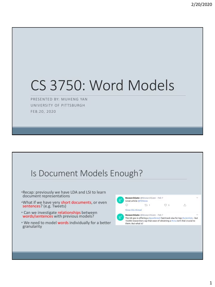
  • What if we have very short documents, or even

sentences? (e.g. Tweets)

  • Can we investigate relationships between

words/sentences with previous models?

  • We need to model words individually for a better

granularity

slide-2
SLIDE 2

2/20/2020 2

Distributional Semantics: from a Linguistic Aspect

Word Embedding, Distributed Representations, Semantic Vector Space... What are they? A more formal term from linguistic: Distributional Semantic Model "… quantifying and categorizing semantic similarities between linguistic items based on their distributional properties in large samples of language data." -- Wikipedia

  • -> Represent elements of language (word here) as distributions of other

elements (i.e. documents, paragraphs, sentences, and words) E.g. word 1 = doc 1 + doc 5 + doc 10 / word 1 = 0.5*word 12 + 0.7*word 24

Document Level Representation

Words as distributions of documents: Latent Semantic Analysis/Indexing (LSA/LSI)

1.Build a co-occurrence matrix of word vs. doc (n by d) 2.Decompose the Word-Document matrix via SVD 3.Take the highest singular values to get the lower-ranked approximation of the w-d matrix, as the word representations

Picture Credit: https://en.wikipedia.org/wiki/Latent_semantic_analysis

slide-3
SLIDE 3

2/20/2020 3

Word Level Representation

  • I. Counting and Matrix Factorization
  • II. Latent Representation

I.Neural Network for Language Models II.CBOW III.Skip-gram IV.Other Models

III.Graph-based Models

I.Node2Vec

Counting and Matrix Factorization

  • Counting methods start with constructing a matrix of co-
  • ccurrences between words and words (can be expanded to other

levels, e.g. at document level it becomes LSA)

  • Due to the high-dimensionality and sparcity, usually used with a

dim-reduction algorithm (PCA, SVD, etc.)

  • The rows of the matrix approximates the distribution of co-
  • ccurring words for every word we are trying to model

Example Models including: LSA, Explicit Semantic Analysis (ESA), Global vectors for word representation (GloVe)

slide-4
SLIDE 4

2/20/2020 4

Explicit Semantic Analysis

  • Similar words most likely appear with the same

distribution of topics

  • ESA represents topics by Wikipedia concepts (Pages).

ESA use Wikipedia concepts as dimensions to construct the space in which words will be projected

  • For each dimension (concept), words in this concept

article are counted

  • Inverted index is then constructed to convert each

word into a vector of concepts

  • The vector constructed for each word represents the

frequency of its occurrences within each (concept).

Picture and Content Credit: Ahmed Magooda

Global vectors for word representation (GloVe)

  • 1. Word-word co-occurrence with sliding

window (|V| by |V|) (and normalize as probability)

  • 2. Construct the cost as:

𝑲 = ෍

𝒋,π’Œ |𝑾|

π’ˆ 𝒀𝒋,π’Œ π’˜π‘—

π‘ˆπ’˜π‘˜ + 𝒄𝑗 + π’„π‘˜ βˆ’ log 𝒀𝑗,π‘˜ πŸ‘

  • 3. Use gradient descent to solve the
  • ptimization

β€œI learn machine learning in CS-3750”

Window=2 I learn machine learning I 1 1 Learn 1 1 1 machine 1 1 2

slide-5
SLIDE 5

2/20/2020 5

GloVe Cont.

How the cost is derived? Probability of word i and k appear together: 𝑄

𝑗,𝑙 = π‘Œπ‘—π‘™ π‘Œπ‘—

Using word k as a probe, the β€œratio” of two word pairs: 𝑠𝑏𝑒𝑗𝑝𝑗,π‘˜,𝑙 =

𝑄𝑗𝑙 π‘„π‘˜π‘™

To model the ratio with embedding v: 𝐾 = Οƒ π‘ π‘π‘’π‘—π‘π‘—π‘˜π‘™ βˆ’ 𝑕 𝑀𝑗, π‘€π‘˜, 𝑀𝑙

2

  • > O(N^3)

Simplify the computation by design 𝑕 βˆ™ = 𝑓 π‘€π‘—βˆ’π‘€π‘˜

π‘ˆπ‘€π‘™

Thus we are trying to make

𝑄𝑗𝑙 π‘„π‘˜π‘™ = 𝑓^(𝑀𝑗

π‘ˆπ‘€π‘™)

𝑓^(π‘€π‘˜

π‘ˆπ‘€π‘™)

Thus we have 𝐾 = Οƒ log 𝑄

π‘—π‘˜ βˆ’ 𝑀𝑗 π‘ˆπ‘€π‘˜ 2

To expand the object log 𝑄

π‘—π‘˜ = 𝑀𝑗 π‘ˆπ‘€π‘˜, we have log π‘Œπ‘—π‘˜ βˆ’ log π‘Œπ‘— = 𝑀𝑗 π‘ˆπ‘€π‘˜, then

log π‘Œπ‘—π‘˜ = 𝑀𝑗

π‘ˆπ‘€π‘˜ + 𝑐𝑗 + 𝑐 π‘˜. By doing this, we solve the problem that 𝑄 π‘—π‘˜ β‰  𝑄 π‘˜π‘—but π‘€π‘˜ π‘ˆπ‘€π‘—

Then we come up with the final cost function 𝐾 = σ𝒋,π’Œ

|𝑾| π’ˆ 𝒀𝒋,π’Œ

π’˜π‘—

π‘ˆπ’˜π‘˜ + 𝒄𝑗 + π’„π‘˜ βˆ’ log 𝒀𝑗,π‘˜ πŸ‘ , where 𝑔(βˆ™) is a weight

function

Value of ratio J and k related J and k not related I and k related 1 Inf I and k not related 1

Latent Representation

Modeling the distribution of context* for a certain words through a series of latent variables, by maximizing the likelihood P(word | context)* Usually fulfilled by neural networks The learned latent variables are used as the representations of words after optimization

* context refers to the other words from the distribution of which we model the target word * in some models it could be P(context | word), e.g. Skip-gram

slide-6
SLIDE 6

2/20/2020 6

Neural Network for Language Model

Learning Objective (predicting next word π’™π’Œ): Find the parameter set πœ„ to minimize 𝑀 πœ„ = βˆ’

1 π‘ˆ Οƒπ‘˜ log(𝑄(π‘₯ π‘˜|π‘₯ π‘˜βˆ’1,… , π‘₯ π‘˜βˆ’π‘œ+1)) + 𝑆(πœ„)

Where 𝑄 βˆ™ =

𝑓𝑧π‘₯𝑗 Οƒπ‘—β‰ π‘˜ 𝑓𝑧π‘₯π‘˜ , Y = b + 𝑿𝑝𝑣𝑒tanh(d + π‘Ώπ‘—π‘œX),

And X is the lookup results of the n-length sequence: X = [𝐷 π‘₯

π‘˜βˆ’1 , … , 𝑑(π‘₯ π‘˜βˆ’π‘œ+1)]

* (𝑿𝑝𝑣𝑒, b) is the parameter set of output layer, (π‘Ώπ‘—π‘œ, d) is the parameter set of hidden layer In this mode we learn the parameters in C (|V| * |N|), π‘Ώπ‘—π‘œ (n * |V| * hidden_size), and 𝑿𝑝𝑣𝑒 (hidden_size * |V|)

Content Credit: Ahmed Magooda

RNN for Language Model

Learning Objective: similar to NN for LM Alter from NN:

  • The hidden layer is now the linear combination of the input

current word t and the hidden of previous word t-1: 𝑑 𝑒 = 𝑔(𝑽π‘₯ 𝑒 + 𝑿𝑑 𝑒 βˆ’ 1 ) Where 𝑔(βˆ™) is the activation function

Content Credit: Ahmed Magooda

slide-7
SLIDE 7

2/20/2020 7

Continuous Bag-of-Words Model

Picture Credit: Francois Chaubard, Rohit Mundra, Richard Socher, from https://cs224d.stanford.edu/lecture_notes/notes1.pdf

Learning Objective: maximizing the likelihood of 𝑄(π‘₯𝑝𝑠𝑒|π‘‘π‘π‘œπ‘’π‘“π‘¦π‘’) for every word in a corpus Similar to NN for LM, the inputs are one-hot vectors and the matrix 𝑿 here is like the look-up matrix. Differences compared to the NN for LM:

  • Bi-directional: not predicting the β€œnext”, instead predicting the center word

inside a window, where words from both directions are input

  • Significantly reduced complexity: only learns 2 * |V| * |N| parameters

CBOW Cont.

Steps breakdown:

  • 1. Generate the one-hot vectors for the context:

(π’šπ‘‘βˆ’π‘›, … , π’šπ‘‘βˆ’1, π’šπ‘‘+1, … , π’šπ‘‘+𝑛 πœ— 𝑺 π‘Š ), and lookup for the word vectors π’˜π‘— = π‘Ώπ’šπ‘—

  • 2. Average the vectors over contexts: π’Šπ‘‘ = π’˜π‘‘βˆ’π‘›+ …+π’˜π‘‘+𝑛

2𝑛

  • 3. Generate the posterior π’œπ‘‘ = π‘Ώβ€²π’Šπ‘‘, and turn it in to

probabilities ෝ 𝒛𝑑 = 𝑑𝑝𝑔𝑒𝑛𝑏𝑦(π’œπ‘‘)

  • 4. Calculate the loss as cross-entropy:σ𝑗=1

|π‘Š| 𝑧𝑗log(ො

𝑧𝑗)  𝑄(π‘₯𝑑|π‘₯π‘‘βˆ’π‘›, … π‘₯𝑑+𝑛) Notations: m: half window size c: center word index π‘₯𝑗: word i from vocabulary V π’šπ‘—: one-hot input of word i π‘Ώπœ— 𝑺 π‘Š Γ— π‘œ: the context lookup matrix π‘Ώβ€²πœ— π‘Ίπ‘œ Γ— π‘Š : the center lookup matrix

slide-8
SLIDE 8

2/20/2020 8

CBOW Cont.

Loss fuction: 𝐺𝑝𝑠 π‘π‘šπ‘š π‘₯𝑑 ∈ π‘Š , π‘›π‘—π‘œπ‘—π‘›π‘—π‘¨π‘“ 𝐾 βˆ™ = π‘šπ‘π‘•π‘„ π‘₯𝑑 π‘₯π‘‘βˆ’π‘›, … π‘₯𝑑+𝑛 β‡’ βˆ’ 1 |π‘Š| ෍ π‘šπ‘π‘•π‘„ 𝑿𝑑 π’Šπ‘‘ = βˆ’ 1 π‘Š ෍ π‘šπ‘π‘• 𝑓𝒙𝑑

β€² π‘ˆ π’Šπ‘‘

Οƒπ‘˜=1

π‘Š π‘“π’™π‘˜

β€²π‘Όπ’Šπ‘‘

= βˆ’ 1 π‘Š ෍ βˆ’π’™π‘‘

β€²π‘ˆπ’Šπ‘‘ + log(෍ π‘˜=1 π‘Š

π‘“π’™π‘˜

β€²π‘Όπ’Šπ‘‘)

Optimization: use SGD to update all relevant vectors 𝒙𝑑

β€² π‘π‘œπ‘’ 𝒙

Skip-gram Model

Picture Credit: Francois Chaubard, Rohit Mundra, Richard Socher, from https://cs224d.stanford.edu/lecture_notes/notes1.pdf

Learning Objective: maximizing the likelihood of 𝑄(π‘‘π‘π‘œπ‘’π‘“π‘¦π‘’|π‘₯𝑝𝑠𝑒) for every word in a corpus Steps Breakdown:

  • 1. Generate one-hot vector for the center word π’š πœ— 𝑺 π‘Š , and calculate the

embedded vector π’Šπ‘‘ = π‘Ώπ’š πœ— π‘Ίπ‘œ

  • 2. Calculate the posterior π’œπ‘‘ = π‘Ώβ€²π’Šπ‘‘
  • 3. For each word j in the context of the center word, calculate the

probabilities ෝ 𝒛𝑑 = 𝑑𝑝𝑔𝑒𝑛𝑏𝑦(π’œπ‘‘)

  • 4. We want the probabilities ො

π‘§π‘‘π‘˜ in ෝ 𝒛𝑑 match the true probabilities of the contexts which are π‘§π‘‘βˆ’π‘›, … , 𝑧𝑑+𝑛

Cost function constructed similarly to the CBOW model

slide-9
SLIDE 9

2/20/2020 9

Skip-gram Cont.

Cost Function: 𝑔𝑝𝑠 𝑓𝑀𝑓𝑠𝑧 π‘‘π‘“π‘œπ‘’π‘“π‘  π‘₯𝑝𝑠𝑒 π‘₯𝑑 π‘—π‘œ π‘Š , π‘›π‘—π‘œπ‘—π‘›π‘—π‘¨π‘“: 𝐾 βˆ™ = βˆ’π‘šπ‘π‘•π‘„ π‘₯π‘‘βˆ’π‘›, … π‘₯𝑑+𝑛 π‘₯𝑑 = βˆ’π‘šπ‘π‘• ΰ·‘

π‘˜=0,π‘˜β‰ π‘› 2𝑛

𝑄 π‘₯π‘‘βˆ’π‘›+π‘˜ π‘₯𝑑 = βˆ’π‘šπ‘π‘• ΰ·‘ 𝑄 π’™π‘‘βˆ’π‘›+π‘˜

β€²

π’Šπ‘‘ = βˆ’ log ΰ·‘ 𝑓𝒙𝑑

β€² π‘ˆ π’Šπ‘‘

Οƒπ‘˜=1

π‘Š π‘“π’™π‘˜

β€²π‘Όπ’Šπ‘‘

Skip-gram with Negative Sampling

An alternative way of learning skip-gram: From the previous learning method, we have looped heavily on negative samples when summing over |V| Alternatively, we can reform the learning objective in order to enabling β€œnegative sampling”, where we only take a few negative samples in each epoch Alternative Objective: maximize the likelihood of P(D=1|w, c) if the word pair (w, c) is from the data, and minimize the likelihood of P(D=0|w, c) if (w, c) is not from the data

slide-10
SLIDE 10

2/20/2020 10

Skip-gram with Negative Sampling

We model the probability as: 𝑄 𝐸 = 1 π‘₯, 𝑑, πœ„ = 𝑑𝑗𝑕𝑛𝑝𝑗𝑒 π’Šπ‘‘

π‘ˆ π’Šπ‘₯ = 𝟐 𝟐+π’‡βˆ’π’Šπ‘‘

π‘ˆ π’Šπ‘₯

And the optimization of the loss would be: πœ„ = argmax

πœ„

Ο‚ π‘₯,𝑑 βˆˆπΈπ‘π‘’π‘ 𝑄 𝐸 = 1 π‘₯, 𝑑, πœ„ Ο‚ π‘₯,𝑑 βˆ‰πΈπ‘π‘’π‘ 𝑄 𝐸 = 0 π‘₯, 𝑑, πœ„ = argmax

πœ„

Ο‚ π‘₯,𝑑 βˆˆπΈπ‘π‘’π‘ 𝑄 𝐸 = 1 π‘₯, 𝑑, πœ„ Ο‚ π‘₯,𝑑 βˆ‰πΈπ‘π‘’π‘(1 βˆ’ 𝑄 𝐸 = 1 π‘₯, 𝑑, πœ„ ) = argmax

πœ„

Οƒ log

1 𝟐+π’‡βˆ’π’Šπ‘‘

π‘ˆ π’Šπ‘₯ Οƒ log(1 βˆ’

1 𝟐+π’‡βˆ’π’Šπ‘‘

π‘ˆ π’Šπ‘₯)

= argmax

πœ„

Οƒ log

1 𝟐+π’‡βˆ’π’Šπ‘‘

π‘ˆ π’Šπ‘₯ Οƒ log

1 𝟐+π’‡π’Šπ‘‘

π‘ˆ π’Šπ‘₯

Hierarchical Softmax and FastText

Hierarchical Softmax: An alternative way to solve the dimensionality problem when softmaxing through y: 1. Build a Binary Tree of words in V, each non-leaf nodes are associated with a pseudo-output to learn. 2. Define the loss for word c as the path to the word from root 3. The probability of 𝑄(π‘₯𝑑|π‘‘π‘π‘œπ‘’π‘“π‘¦π‘’) now becomes Ο‚π‘˜=1

π‘šπ‘“π‘œπ‘•π‘’β„Ž 𝑝𝑔 π‘žπ‘π‘’β„Ž 𝑑𝑗𝑕𝑛𝑝𝑗𝑒( π‘œ π‘₯, π‘˜ + 1 𝑗𝑑 π‘’β„Žπ‘“ π‘‘β„Žπ‘—π‘šπ‘’π‘“π‘ π‘œ βˆ™ π’Š π‘₯,π‘˜ π‘ˆ

π’Šπ‘‘) FastText: Sub-word n-grams + Hierarchical Softmax β€œapple” and β€œapples” are referring to the same semantic, yet word model ignores such sub-word features. FastText model introduces sub-word n-gram inputs, while having a similar architecture as skip-gram models. This expands the dimension of 𝒛 to a even larger number. Thus it adopts the Hierarchical Softmax to speed up the computation

slide-11
SLIDE 11

2/20/2020 11

Graph-based Models

WordNet:

A large lexical database of words. Words are grouped into set of synonyms (synsets), each expressing a distinct concept Provides Word senses, Part of Speech, semantic relationships between words From which we can construct a real β€œnet” of words where words are nodes and word relationships defined by synsets as edges

Content Credit: Ahmed Magooda

Node2Vec

A model to learn representations

  • f nodes:

Applied to any graphs including word nets Turns graph topology into sequences with the random walk algorithm: Start from a random node v, the probability of travel to another node is: 𝑄 𝑦 𝑀 = ࡝

πœŒπ‘€π‘¦ π‘Ž 𝑗𝑔 𝑀, 𝑦 ∈ 𝐹

0 π‘π‘’β„Žπ‘“π‘ π‘₯𝑗𝑑𝑓 The transition probability is defined as: πœŒπ‘€π‘¦ = 1 π‘ž 𝑗𝑔 𝑦 𝑗𝑑 π‘’β„Žπ‘“ π‘žπ‘ π‘“π‘€π‘—π‘π‘£π‘‘ π‘œπ‘π‘’π‘“ 𝑒 1 𝑗𝑔 𝑦 𝑗𝑑 π‘’β„Žπ‘“ π‘œπ‘“π‘—π‘•β„Žπ‘π‘π‘  𝑝𝑔 𝑒 1 π‘Ÿ 𝑗𝑔 𝑦 𝑗𝑑 π‘œπ‘“π‘—π‘•β„Žπ‘π‘π‘  𝑝𝑔 π‘œπ‘“π‘—π‘•β„Žπ‘π‘π‘  𝑝𝑔 𝑒 p and q controls the strategy of breath-first search or depth-first search With the sequence generated, we can embed nodes as we did in language models

slide-12
SLIDE 12

2/20/2020 12

Evaluation of Word Representations

  • Intrinsic Evaluation:
  • How good are the representations?
  • Extrinsic Evaluation:
  • How effective are the learned representations in other

downstream tasks?

Content Credit: Ahmed Magooda

Intrinsic Evaluations

Word Similarity Task

  • Calculate the similarity of word pairs from the learned vectors through a various distance metrics (e.g.

euclidean, cosine, etc.)

  • Compare the calculated word similarities with human-annotated similarities
  • Example test set: word-sim 353 (http://www.cs.technion.ac.il/~gabr/resources/data/wordsim353/)

Analogy Task:

  • Proposed by Mikolov et.al (2013)
  • For a specific word relation, given a, b, y; find x so

that "a is to b as x is to y"

  • "man is to king as woman is to queen"

"Analogy task" Content Credit: Ahmed Magooda

slide-13
SLIDE 13

2/20/2020 13

Extrinsic Evaluations

Learned word representations can be taken as inputs to encode texts in downstream NLP tasks, including:

  • Sentiment Analysis, POS tagging, QA, Machine

Translation...

  • GLUE benchmark: a collection of dataset including 9

sentence language understanding tasks (https://gluebenchmark.com/)

Summary

What we have covered:

  • "words as distributions"
  • evaluations of the word representations

Document-level Word-level Count & Decomposition

  • LSA
  • GloVe

Latent Vector Representation

  • NN for LM
  • CBOW, Skip-gram, FastText
  • Node2Vec
slide-14
SLIDE 14

2/20/2020 14

Software at Fingertips

LSA : manual through sklearn or Gensim CBOW, Skip-gram: Gensim Neural-networks: Torch, Tensorflow Pre-trained word representations:

  • Word2vec: (https://drive.google.com/file/d/0B7XkCwpI5KDYNlNUTTlSS21pQmM/edit)
  • Glove: (https://nlp.stanford.edu/projects/glove/)
  • Fasttext: (https://fasttext.cc/)

References

Word2Vec:

  • Mikolov, T., Chen, K., Corrado, G., & Dean, J. (2013). Efficient estimation of word representations in vector space.
  • Mikolov, T., Sutskever, I., Chen, K., Corrado, G. S., & Dean, J. (2013). Distributed representations of words and phrases and their compositionality.
  • Mikolov, T., Yih, W. T., & Zweig, G. (2013, June). Linguistic Regularities in Continuous Space Word Representations.
  • Bojanowski, P., Grave, E., Joulin, A., & Mikolov, T. (2017). Enriching word vectors with subword information. Transactions of the Association for Computational Linguistics, 5, 135-146.

Counting:

  • Pennington, J., Socher, R., & Manning, C. D. (2014, October). Glove: Global vectors for word representation. In Proceedings of the 2014 conference on empirical methods in natural language processing

(EMNLP) (pp. 1532-1543).

  • Gabrilovich, E., & Markovitch, S. (2007, January). Computing semantic relatedness using wikipedia-based explicit semantic analysis.
  • Deerwester, S., Dumais, S. T., Furnas, G. W., Landauer, T. K., & Harshman, R. (1990). Indexing by latent semantic analysis.

NN for LM:

  • Mikolov, T., Kopecky, J., Burget, L., & Glembek, O. (2009, April). Neural network based language models for highly inflective languages.
  • Mikolov, T., KarafiΓ‘t, M., Burget, L., ČernockΓ½, J., & Khudanpur, S. (2010). Recurrent neural network based language model.

Graph-based:

  • Princeton University "About WordNet." WordNet. Princeton University. 2010. http://wordnet.princeton.edu
  • Grover, A., & Leskovec, J. (2016, August). node2vec: Scalable feature learning for networks. In Proceedings of the 22nd ACM SIGKDD international conference on Knowledge discovery and data

mining (pp. 855-864).