CS4100 Outline CS 4100: Artificial Intelligence We Were re done - - PowerPoint PPT Presentation

SLIDE 1

CS4100 Outline

• We

We’re re done

• ne with

h Part art I: Search earch and and Planni anning ng!

• Part II: Probabilist

stic Reaso soning

• Diagnosi

sis

• Spe

Speech r recogn gniti tion

• Tracki

king objects

• Ro

Robot mapping

• Ge

Geneti tics

• Er

Error c correcti ting c g code des

• …

… lots s more!

• Pa

Part III: Machine Learning

CS 4100: Artificial Intelligence Probability

Jan-Willem van de Meent, Northeastern University

[These slides were created by Dan Klein and Pieter Abbeel for CS188 Intro to AI at UC Berkeley. All CS188 materials are available at http://ai.berkeley.edu.]

Today

• Pr

Proba babi bility

• Ra

Random Variables

• Jo

Joint and Marginal Dist stributions

• Conditional Dist

stribution

• Product Rule, Chain Rule, Baye

yes’ s’ Rule

• In

Infe ference

• In

Inde depe pende dence

• Yo

You’ll need d all this s st stuff A LOT fo for th the next xt few weeks, ks, so so make ke su sure yo you go go

• ve

ver it now!

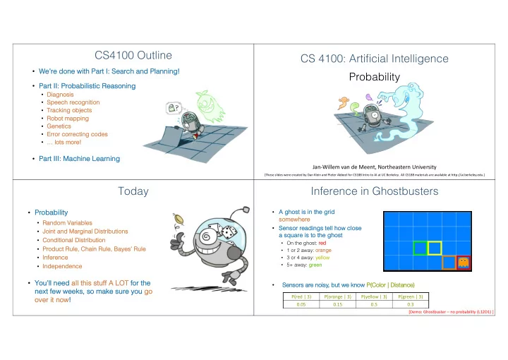
Inference in Ghostbusters

• A ghost

st is s in the grid so somewhere

• Senso

sor readings s tell how close se a sq square is s to the ghost st

• On the ghost: re

red

• 1 or 2 away: or
• rang

ange

• 3 or 4 away: ye

yellow

• 5+ away: gr

green P(red | 3) P(orange | 3) P(yellow | 3) P(green | 3) 0.05 0.15 0.5 0.3

• Sensors are noisy, but we kn

know P( P(Color | Distance)

[Demo: Ghostbuster – no probability (L12D1) ]

SLIDE 2

Ghostbusters Uncertainty

• General si

situation:

• Obse

serve ved va variables s (evi vidence): Agent knows certain things about the state of the world (e.g., sensor readings or symptoms)

• Unobse

serve ved va variables: s: Agent needs to reason about other aspects (e.g. where an object is or what disease is present)

• Mo

Model: Agent knows something about how the known variables relate to the unknown variables

• Probabilist

stic reaso soning give ves s us s a framework k for managing our beliefs s and kn knowledge

Random Variables

• A

A random va variable is s so some asp spect of the world about which we (may) y) have ve uncertainty

• R = Is

s it raining?

• T = Is

s it hot or cold?

• D = How long will it take

ke to drive ve to work?

• L = Where is

s the ghost st?

• We

We denot enote e random va variables s wit with cap capital al let etter ers

• Like

ke va variables s in a CSP, random va variables s have ve domains

• R in {true, false

se} (often write as {+ {+r, r, -r} r})

• T in {h

{hot, cold}

• D in [0

[0, ¥)

• L in possible locations, maybe {(0,0), (0,1), …}

…}

Probability Distributions

• Asso

ssociate a probability y with each va value

T P hot 0.5 cold 0.5 W P sun 0.6 rain 0.1 fog 0.3 meteor 0.0

Te Temperature We Weather

SLIDE 3

Shorthand notation: OK if all domain entries are unique

Probability Distributions

• Unobse

serve ved random va variables s have ve dist stributions

• Think

k of a dist stribution as s a ta tabl ble of

• f pr

proba babi biliti ties

• Think

k of probability y (lower case se va value) as s a si single entry y in this s table

• Must

st have ve: and

T P hot 0.5 cold 0.5 W P sun 0.6 rain 0.1 fog 0.3 meteor 0.0

Joint Distributions

• A

A joint dist stribution ove ver a se set of random va variables: s: sp specifies s a real number for each assi ssignment (or out

• utcom

come): ):

• Must obey:
• Size

ze of dist stribution of

• f n

n va variables s with domain si size zes s d?

• For all but the smallest distributions, impractical to write out!

T W P hot sun 0.4 hot rain 0.1 cold sun 0.2 cold rain 0.3

An Answer: dn

Probabilistic Models

• A

A probabilist stic model is s a joint dist stribution ove ver a se set of random va variables

• Probabilist

stic models: s:

• Random

Random va variables s with domains

• Assignments are called outcom
• utcomes

es

• Jo

Joint dist stributions: s: say whether assignments (outcomes) are likely

• Normalize

zed: sum to 1.0

• Ideally:

y: only certain variables directly interact

• Const

straint sa satisf sfaction problems: s:

• Variables

s with domains

• Const

straints: s: state whether assignments are possible

• Ideally:

y: only certain variables directly interact

T W P hot sun 0.4 hot rain 0.1 cold sun 0.2 cold rain 0.3 T W P hot sun T hot rain F cold sun F cold rain T

Distribution over T, W Constraint over T, W

Events

• An

An eve vent is s a se set E of

• f out
• utcomes

comes

• From a joint dist

stribution, we can cal calcul culat ate e th the probability y of any y eve vent

• Probability that it’s hot AND su

sunny?

• Probability that it’s hot

hot?

• Probability that it’s hot OR su

sunny?

• Typ

ypically, y, the eve vents s we care about are partial assi ssignments, like ke P( P(T=h =hot)

T W P hot sun 0.4 hot rain 0.1 cold sun 0.2 cold rain 0.3

SLIDE 4

Quiz: Events

• P(+x,

x, +y) y) ?

• P(+x)

x) ?

• P(

P(-y y OR +x) x) ?

X Y P +x +y 0.2 +x

• y

0.3

• x

+y 0.4

• x
• y

0.1

0. 0.2 0. 0.5 0. 0.6

Marginal Distributions

• Marginal dist

stributions ar are e “su sub-tables” s” which eliminate va variables s

• Marginaliza

zation (su summing out): Combine collapse sed rows s by y adding T W P hot sun 0.4 hot rain 0.1 cold sun 0.2 cold rain 0.3 T P hot 0.5 cold 0.5 W P sun 0.6 rain 0.4

Quiz: Marginal Distributions

X Y P +x +y 0.2 +x

• y

0.3

• x

+y 0.4

• x
• y

0.1 X P +x

• x

Y P +y

• y

0.5 0.5 0.6 0.4

Conditional Probabilities

• A si

simple relation between jo join int and and cond conditional

• nal prob
• bab

abilities es

• In fact, this is taken as the de

definition of a cond conditional

• nal prob
• bab

ability T W P hot sun 0.4 hot rain 0.1 cold sun 0.2 cold rain 0.3 P(b) P(a) P(a,b)

SLIDE 5

Quiz: Conditional Probabilities

• P(+x

x | +y) y) ?

• P(

P(-x x | +y) y) ?

• P(

P(-y y | +x) x) ?

X Y P +x +y 0.2 +x

• y

0.3

• x

+y 0.4

• x
• y

0.1

0. 0.2 / (0 (0.2 + 0. 0.4) 4) = 0. 0.33 0. 0.4 4 / (0 (0.2 + 0. 0.4) 4) = 0. 0.66 66 = = 1- 0. 0.33 33 0. 0.3 3 / (0 (0.2 + 0. 0.3) 3) = 0. 0.6

Conditional Distributions

• Conditional dist

stributions are probability y dist stributions s

• ve

ver so some va variables s give ven fixe xed va values s of others

T W P hot sun 0.4 hot rain 0.1 cold sun 0.2 cold rain 0.3 W P sun 0.8 rain 0.2 W P sun 0.4 rain 0.6

Conditional Distributions Joint Distribution

Normalization Trick

T W P hot sun 0.4 hot rain 0.1 cold sun 0.2 cold rain 0.3 W P sun 0.4 rain 0.6 SELECT the joint probabilities matching the evidence

Normalization Trick

T W P hot sun 0.4 hot rain 0.1 cold sun 0.2 cold rain 0.3 W P sun 0.4 rain 0.6 T W P cold sun 0.2 cold rain 0.3 NORMALIZE the selection (make it sum to one)

SLIDE 6

Normalization Trick

• Why does this work? Sum of selection is P(evi

vidence)! (here P(T (T=c))

T W P hot sun 0.4 hot rain 0.1 cold sun 0.2 cold rain 0.3 W P sun 0.4 rain 0.6 T W P cold sun 0.2 cold rain 0.3 SELECT the joint probabilities matching the evidence NORMALIZE the selection (make it sum to one)

Quiz: Normalization Trick

• P(

P(X X | Y= Y=-y) y) ?

X Y P +x +y 0.2 +x

• y

0.3

• x

+y 0.4

• x
• y

0.1 SELECT the joint probabilities matching the evidence NORMALIZE the selection (make it sum to one) X Y P

• y

+x 0.3

• y
• x

0.1 X Y P

• y

+x 0.75

• y
• x

0.25

To Normalize

• (Dictionary)

y) To bring or rest store to a nor normal al cond condition

• n
• Pr

Procedu dure:

• St

Step p 1: Compute Z = su sum ove ver all entries

• St

Step p 2: Divide every entry by Z

All entries sum to ONE

W P sun 0.2 rain 0.3

Z = 0.5

W P sun 0.4 rain 0.6

T W P hot sun 20 hot rain 5 cold sun 10 cold rain 15 Normalize Z = 50 Normalize T W P hot sun 0.4 hot rain 0.1 cold sun 0.2 cold rain 0.3

Ex Examp mple 1 Ex Examp mple 2

Probabilistic Inference

• Probabilist

stic inference: compute a desired probability from other known probabilities (e.g. conditional from joint)

• We generally

y compute conditional probabilities s

• P(on time | no reported accidents)

s) = 0.90

• These represent the agent’s beliefs

s given the evi vidence

• Probabilities

s change with new evi vidence:

• P(on time | no accidents,

s, 5 a.m.) = 0.95

• P(on time | no accidents,

s, 5 a.m., raining) = 0.80

• Additional evidence causes beliefs

s to be updated

SLIDE 7

Inference by Enumeration

• General case

se:

• Evi

vidence variables:

• Query*

y* variable:

• Hidde

Hidden variables: All variables

* Works fine with multiple query variables, too

We want: Step 1: Select the entries consistent with evidence Step 2: Sum out H to get joint

• f query and evidence

Step 3: Normalize

× 1 Z

Inference by Enumeration

• P(

P(W)?

• P(

P(W | | win winter)?

• P(

P(W | | win winter, hot)?

S T W P summer hot sun 0.30 summer hot rain 0.05 summer cold sun 0.10 summer cold rain 0.05 winter hot sun 0.10 winter hot rain 0.05 winter cold sun 0.15 winter cold rain 0.20 W P sun 0.3 + 0.1 + 0.1 + 0.15 = 0.65 rain 0.05 + 0.05 + 0.05 + 0.2 = 0.35

Inference by Enumeration

• P(

P(W)?

• P(

P(W | | win winter)?

• P(

P(W | | win winter, hot)?

S T W P summer hot sun 0.30 summer hot rain 0.05 summer cold sun 0.10 summer cold rain 0.05 winter hot sun 0.10 winter hot rain 0.05 winter cold sun 0.15 winter cold rain 0.20 W P sun 0.3 + 0.1 + 0.1 + 0.15 = 0.65 rain 0.05 + 0.05 + 0.05 + 0.2 = 0.35 W P sun 0.1+0.15 = 0.25 rain 0.05+0.2 = 0.25 W P sun 0.5 rain 0.5

Inference by Enumeration

• P(

P(W)?

• P(

P(W | | win winter)?

• P(

P(W | | win winter, hot)?

S T W P summer hot sun 0.30 summer hot rain 0.05 summer cold sun 0.10 summer cold rain 0.05 winter hot sun 0.10 winter hot rain 0.05 winter cold sun 0.15 winter cold rain 0.20 W P sun 0.3 + 0.1 + 0.1 + 0.15 = 0.65 rain 0.05 + 0.05 + 0.05 + 0.2 = 0.35 W P sun 0.1+0.15 = 0.25 rain 0.05+0.2 = 0.25 W P sun 0.5 rain 0.5 W P sun 0.1 rain 0.05 W P sun 0.66 rain 0.33

SLIDE 8

• Obv

Obvious pr probl blems:

• Wo

Worst-case case time e com complex exity y O( O(dn) )

• Spa

Space compl plexity O( O(dn) to to sto tore th the joint t distri tributi tion

Inference by Enumeration The Product Rule

• Sometimes

s we have ve conditional dist stributions s bu but w t want th t the jo join int

The Product Rule

• Example:

R P sun 0.8 rain 0.2 D W P wet sun 0.1 dry sun 0.9 wet rain 0.7 dry rain 0.3 D W P wet sun 0.08 dry sun 0.72 wet rain 0.14 dry rain 0.06

The Chain Rule

• More generally,

y, can always ys write any y joint dist stribution as s an incremental product of conditional dist stributions

• Why

y is s this s always ys true?

SLIDE 9

Bayes’ Rule Bayes’ Rule

• Two ways

ys to factor a joint dist stribution ove ver two va variables: s:

• Divi

viding, w , we ge get: t:

• Why

y is s this s at all helpful?

• Lets us build one cond

conditional

• nal from its reve

verse se

• Often one conditional is tricky but the other one is simple
• Foundation of many systems we’ll see later (e.g. ASR, MT)
• In the running for most

st important AI equation!

* this may not be Thomas Bayes ** Bayes’ rule was published posthumously by Richard Price, and was ignored until work by Laplace

Inference with Bayes’ Rule

• Exa

xample: Diagnost stic probability y from causa sal pr proba babi bility ty

• M:

M: me meningitis, S: S: st stiff neck

• No

Note te: posterior probability of meningitis still very small

• No

Note te: you should still get stiff necks checked out! Why?

Example givens

P(+s| − m) = 0.01

) = P(+s| + m)P(+m) P(+s| + m)P(+m) + P(+s| − m)P(−m)

P(+m) = 0.0001 P(+s| + m) = 0.8 P(cause|effect) = P(effect|cause)P(cause) P(effect)

P(+m| + s) = P(+s| + m)P(+m) P(+s) ) = 0.8 × 0.0001 0.8 × 0.0001 + 0.01 × 0.9999 = 0.0079

Ghostbusters, Revisited

• Let’s

s sa say y we have ve two dist stributions: s:

• Prior dist

stribution over ghost location P( P(G)

• Let’s say this is uniform
• Senso

sor reading model P( P(R R | G)

• Give

ven: we know what our sensors do

• R = reading color measu

sured at (1,1)

• E.g. P(R = ye

yellow | G=(1,1)) = 0.1

• We

We can can calculat calculate e the he post sterior dist stribution P( P(G | G | r r) ove ver ghost st locations s give ven a re reading

[Demo: Ghostbuster – with probability (L12D2) ]

SLIDE 10

Ghostbusters with Probability Next Time: Markov Models