CS70: Jean Walrand: Lecture 23. Probability Basics Review Exactly - - PowerPoint PPT Presentation

CS70: Jean Walrand: Lecture 23.

What do we learn from observations?

• 1. Probability Basics Review
• 2. Examples
• 3. Conditional Probability

Probability Basics Review

Setup:

◮ Random Experiment.

Flip a coin twice.

◮ Probability Space.

◮ Sample Space: Set of outcomes, Ω.

Ω = {HH,HT,TH,TT}

◮ Probability: Pr[ω] for all ω ∈ Ω.

Pr[HH] = ··· = Pr[TT] = 1/4

• 1. 0 ≤ Pr[ω] ≤ 1.
• 2. ∑ω∈Ω Pr[ω] = 1.

◮ Event: A ⊆ Ω,Pr[A] = ∑ω∈Ω Pr[ω].

Pr[at least one H out of two tosses] = Pr[HT,TH,HH] = 3/4

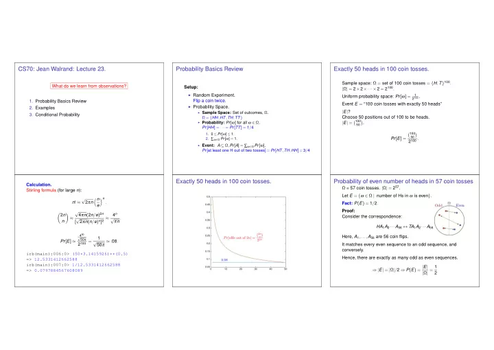
Exactly 50 heads in 100 coin tosses.

Sample space: Ω = set of 100 coin tosses = {H,T}100. |Ω| = 2×2×···×2 = 2100. Uniform probability space: Pr[ω] =

1 2100 .

Event E = “100 coin tosses with exactly 50 heads” |E|? Choose 50 positions out of 100 to be heads. |E| = 100

50

• .

Pr[E] = 100

50

• 2100 .

Calculation. Stirling formula (for large n): n! ≈ √ 2πn n e n . 2n n

• ≈

√ 4πn(2n/e)2n [ √ 2πn(n/e)n]2 ≈ 4n √πn. Pr[E] ≈

450 √ 50π

2100 = 1 √ 50π ≈ .08. irb(main):006:0> (50*3.1415926)**(0.5) => 12.5331412662588 irb(main):007:0> 1/12.5331412662588 => 0.0797884567608089

Exactly 50 heads in 100 coin tosses. Probability of even number of heads in 57 coin tosses

Ω = 57 coin tosses. |Ω| = 257. Let E = {ω ∈ Ω | number of Hs in ω is even}. Fact: P(E) = 1/2. Proof: Consider the correspondence: HA1A2 ···A56 ↔ TA1A2 ···A56 Here, A1,...,A56 are 56 coin flips. It matches every even sequence to an odd sequence, and conversely. Hence, there are exactly as many odd as even sequences. ⇒ |E| = |Ω|/2 ⇒ P(E) = |E| |Ω| = 1 2

Probability more heads than tails in 100 coin tosses.

Ω = 100 coin tosses. |Ω| = 2100. Recall event E = ‘equal heads and tails’ Event F = ‘more heads than tails’ Event G = ‘more tails than heads’ A 1-to-1 correspondence between

• utcomes in F and G!

|F| = |G|. E, F and G are disjoint. Pr[E] ≈ 8%. |Ω| = |E|+|F|+|G|. ⇒ 1 = Pr[Ω] = Pr[E]+2Pr[F] ≈ 8%+2Pr[F]. Solve for |F|: |F| ≈ 46%

Probability of n heads in 100 coin tosses.

Ω = 100 coin tosses. |Ω| = 2100. Event En = ‘n heads’; |En| = 100

n

• n

p n

pn = Pr[En] = |En| |Ω| = 100

n

• 2100

Roll a red and a blue die.

Ω = {(a,b) : 1 ≤ a,b ≤ 6} = {1,2,...,6}2. Uniform: Pr[ω] =

1 |Ω| = 1 36 for all ω.

What is the probability of

• 1. the red die showing 6?

E1 = {(6,b) : 1 ≤ b ≤ 6}, |E1| = 6, Pr[E1] = |E1|/|Ω| = 1/6

• 2. at least one die showing 6?

E1 = {(6,b) : 1 ≤ b ≤ 6} = red die shows 6 E2 = {(a,6) : 1 ≤ a ≤ 6} = blue die shows 6 E = E1 ∪E2 = red or blue die (or both) show 6 |E| = |E1|+|E2|−|E1 ∩E2| [Inclusion/Exclusion] |E1 ∩E2| = {(6,6)} |E| = 6+6−1 = 11 Pr[E] = 11/36

Roll a red and a blue die.

E1 = ‘Red die shows 6’;E2 = ‘Blue die shows 6’ E1 ∪E2 = ‘At least one die shows 6’ Pr[E1] = 6 36,Pr[E2] = 6 36,Pr[E1 ∪E2] = 11 36.

Inclusion/Exclusion

Note that, Pr[A∪B] = Pr[A]+Pr[B]−Pr[A∩B] whether or not the sample space has uniform distribution.

Roll a red and a blue die.

Ω = {(a,b) : 1 ≤ a,b ≤ 6} = {1,2,...,6}2. Uniform: Pr[ω] =

1 |Ω| = 1 36 for all ω.

What is the probability of

• 1. the dice sum to 7?

E = {(1,6),(2,5),(3,4),(4,3),(5,2),(6,1)};|E| = 6. Counting argument: for each choice a of the value of the red die, there is exactly one choice b = 7−a for the blue die, so there are 6 total choices. Pr[E] = |E|/|Ω| = 6/36 = 1/6.

• 2. the dice sum to 10?

E = {(4,6),(5,5),(6,4)} Pr[E] = |E|/|Ω| = 3/36 = 1/12.

Roll a red and a blue die. Roll two blue dice.

The key idea is that we do not distinguish the dice. Roll die 1, then die 2. Then forget the order. For instance, we consider that (2,5) and (5,2) are the same

• utcome.

We designate this outcome by (2,5). Thus, Ω′ = {(a,b) | 1 ≤ a ≤ b ≤ 6}. We see that Pr[(1,3)] = 2

36 and Pr[(2,2)] = 1 36.

Roll two blue dice

Two different models of the same random experiment. In Ω′,Pr[(1,3)] = 2 36 and Pr[(2,2)] = 1 36

Roll two blue dice.

Now what is the probability of at least one die showing 6? In Ω,Pr[A] = 11

36; in Ω′,Pr[B] = 5× 2 36 +1× 1 36.

Of course, this is the same as for distinguishable dice! The event does not depend on the dice being distinguishable.

Roll two blue dice.

What is the probability of the dice sum to 7? In Ω,Pr[A] = 6

36; in Ω′,Pr[B] = 3× 2 36.

Of course, this is the same as for distinguishable dice! The event does not depend on the dice being distinguishable.

Really not uniform! and not finite!

◮ Experiment: Toss three times a coin with Pr[H] = 2/3.

◮ Ω = {HHH,HHT,HTH,HTT,THH,THT,TTH,TTT}. ◮ Pr[HHH] = ( 2

3)3; Pr[HHT] = ( 2 3)2( 1 3); . . . ◮ Toss a fair coin until you get a heads.

◮ Ω = {H,TH,TTH,TTTH,...} ◮ Pr[H] = 1

2,Pr[TH] = 1 4,Pr[TTH] = 1 8

◮ Still sums to 1. Indeed 1

2 + 1 4 + 1 8 + 1 16 +··· = 1.

Set notation review

A B Ω

Figure : Two events

Ω ¯ A

Figure : Complement (not)

Ω A [ B

Figure : Union (or)

Ω A ∩ B

Figure : Intersection (and)

Ω A \ B

Figure : Difference (A, not B)

Ω A ∆B

Figure : Symmetric difference (only one)

Conditional probability: example.

Two coin flips. First flip is heads. Probability of two heads? Ω = {HH,HT,TH,TT}; Uniform probability space. Event A = first flip is heads: A = {HH,HT}. New sample space: A; uniform still. Event B = two heads. The probability of two heads if the first flip is heads. The probability of B given A is 1/2.

A similar example.

Two coin flips. One of the flips is heads. Probability of two heads? Ω = {HH,HT,TH,TT}; uniform. Event A = one flip is heads. A = {HH,HT,TH}. New sample space: A; uniform still. Event B = two heads. The probability of two heads if at least one flip is heads. The probability of B given A is 1/3.

Conditional Probability: A non-uniform example

Consider Ω = {1,2,...,N} with Pr[n] = pn. Pr[3|B] = p3 p1 +p2 +p3 = p3 Pr[B]. ω / ∈ B ⇒ Pr[ω|B] = 0.

Another non-uniform example

Consider Ω = {1,2,...,N} with Pr[n] = pn. Pr[A|B] = p3 p1 +p2 +p3 = Pr[A∩B] Pr[B] .

Yet another non-uniform example

Consider Ω = {1,2,...,N} with Pr[n] = pn. Pr[A|B] = p2 +p3 p1 +p2 +p3 = Pr[A∩B] Pr[B] .

Conditional Probability.

If in A, what is the probability of outcome ω? If ω ∈ A, probability is 0 Otherwise: Ratio of probability of ω to total probability of A Pr[ω|A] = Pr[ω] Pr[A] Uniform Probability Space: Ratio of 1/|Ω| to |A|/|Ω| = ⇒ 1/|A|. (Makes sense!)

Conditional Probability.

Definition: The conditional probability of B given A is Pr[B|A] = ∑

ω∈B

Pr[ω|A] = ∑ω∈A∩B Pr[ω] Pr[A] = Pr[A∩B] Pr[A]

Conditional Probability.

Definition: The conditional probability of B given A is Pr[B|A] = Pr[A∩B] Pr[A] A B A B In A! In B? Must be in A∩B. A∩B Pr[B|A] = Pr[A∩B]

Pr[A] .

What do we learn from observations? You observe that the event B occurs. That changes your information about the probability of every event A. The conditional probability of A given B is Pr[A|B] = Pr[A∩B] Pr[B] . Note: Pr[A∩B] = Pr[B]×Pr[A|B] = Pr[A]×Pr[B|A].