SLIDE 1 CSE 373: Disjoint sets
Michael Lee Wednesday, Feb 28, 2018
1
Review Last time... ◮ Prim’s algorithm: Nearly identical to Dijkstra’s, except we use the distance to any already-visited node as the cost. ◮ Kruskal’s algorithm: Loop over edges, from smallest to largest. Use the edge only if it doesn’t introduce a cycle.
2
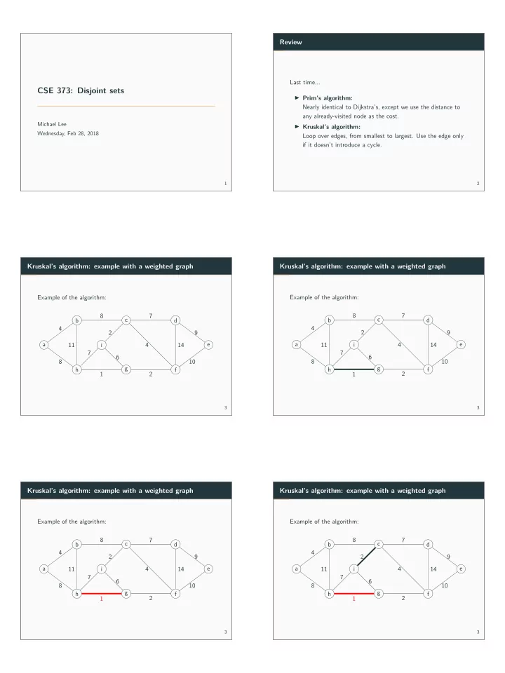
Kruskal’s algorithm: example with a weighted graph Example of the algorithm: a b c d e f g h i 4 8 8 11 7 4 2 9 14 10 2 1 6 7
3
Kruskal’s algorithm: example with a weighted graph Example of the algorithm: a b c d e f g h i 4 8 8 11 7 4 2 9 14 10 2 1 6 7
3
Kruskal’s algorithm: example with a weighted graph Example of the algorithm: a b c d e f g h i 4 8 8 11 7 4 2 9 14 10 2 1 6 7
3
Kruskal’s algorithm: example with a weighted graph Example of the algorithm: a b c d e f g h i 4 8 8 11 7 4 2 9 14 10 2 1 6 7
3
SLIDE 2 Kruskal’s algorithm: example with a weighted graph Example of the algorithm: a b c d e f g h i 4 8 8 11 7 4 2 9 14 10 2 1 6 7
3
Kruskal’s algorithm: example with a weighted graph Example of the algorithm: a b c d e f g h i 4 8 8 11 7 4 2 9 14 10 2 1 6 7
3
Kruskal’s algorithm: example with a weighted graph Example of the algorithm: a b c d e f g h i 4 8 8 11 7 4 2 9 14 10 2 1 6 7
3
Kruskal’s algorithm: example with a weighted graph Example of the algorithm: a b c d e f g h i 4 8 8 11 7 4 2 9 14 10 2 1 6 7
3
Kruskal’s algorithm: example with a weighted graph Example of the algorithm: a b c d e f g h i 4 8 8 11 7 4 2 9 14 10 2 1 6 7
3
Kruskal’s algorithm: example with a weighted graph Example of the algorithm: a b c d e f g h i 4 8 8 11 7 4 2 9 14 10 2 1 6 7
3
SLIDE 3 Kruskal’s algorithm: example with a weighted graph Example of the algorithm: a b c d e f g h i 4 8 8 11 7 4 2 9 14 10 2 1 6 7
3
Kruskal’s algorithm: example with a weighted graph Example of the algorithm: a b c d e f g h i 4 8 8 11 7 4 2 9 14 10 2 1 6 7
3
Kruskal’s algorithm: example with a weighted graph Example of the algorithm: a b c d e f g h i 4 8 8 11 7 4 2 9 14 10 2 1 6 7
3
Kruskal’s algorithm: example with a weighted graph Example of the algorithm: a b c d e f g h i 4 8 8 11 7 4 2 9 14 10 2 1 6 7
3
Kruskal’s algorithm: example with a weighted graph Example of the algorithm: a b c d e f g h i 4 8 8 11 7 4 2 9 14 10 2 1 6 7
3
Kruskal’s algorithm: example with a weighted graph Example of the algorithm: a b c d e f g h i 4 8 8 11 7 4 2 9 14 10 2 1 6 7
3
SLIDE 4 Kruskal’s algorithm: example with a weighted graph Example of the algorithm: a b c d e f g h i 4 8 8 11 7 4 2 9 14 10 2 1 6 7
3
Kruskal’s algorithm: example with a weighted graph Example of the algorithm: a b c d e f g h i 4 8 8 11 7 4 2 9 14 10 2 1 6 7
3
Kruskal’s algorithm: example with a weighted graph Example of the algorithm: a b c d e f g h i 4 8 8 11 7 4 2 9 14 10 2 1 6 7
3
Kruskal’s algorithm: example with a weighted graph Example of the algorithm: a b c d e f g h i 4 8 8 11 7 4 2 9 14 10 2 1 6 7
3
Kruskal’s algorithm: example with a weighted graph Example of the algorithm: a b c d e f g h i 4 8 8 11 7 4 2 9 14 10 2 1 6 7
3
Kruskal’s algorithm: example with a weighted graph Example of the algorithm: a b c d e f g h i 4 8 8 11 7 4 2 9 14 10 2 1 6 7
3
SLIDE 5 Kruskal’s algorithm: example with a weighted graph Example of the algorithm: a b c d e f g h i 4 8 8 11 7 4 2 9 14 10 2 1 6 7
3
Kruskal’s algorithm: example with a weighted graph Example of the algorithm: a b c d e f g h i 4 8 8 11 7 4 2 9 14 10 2 1 6 7
3
Kruskal’s algorithm: example with a weighted graph Example of the algorithm: a b c d e f g h i 4 8 8 11 7 4 2 9 14 10 2 1 6 7
3
Kruskal’s algorithm: example with a weighted graph Example of the algorithm: a b c d e f g h i 4 8 8 11 7 4 2 9 14 10 2 1 6 7
3
Kruskal’s algorithm: example with a weighted graph Example of the algorithm: a b c d e f g h i 4 8 8 11 7 4 2 9 14 10 2 1 6 7
3
Kruskal’s algorithm: example with a weighted graph Example of the algorithm: a b c d e f g h i 4 8 8 11 7 4 2 9 14 10 2 1 6 7
3
SLIDE 6 Kruskal’s algorithm: example with a weighted graph Example of the algorithm: a b c d e f g h i 4 8 8 11 7 4 2 9 14 10 2 1 6 7
3
Kruskal’s algorithm: analysis Runtime analysis:
def kruskal(): for (v : vertices): makeMST(v) sort edges in ascending order by their weight mst = new SomeSet<Edge>() for (edge : edges): if findMST(edge.src) != findMST(edge.dst): union(edge.src, edge.dst) mst.add(edge) return mst
Note: assume that... ◮ makeMST(v) takes O (tm) time ◮ findMST(v): takes O (tf ) time ◮ union(u, v): takes O (tu) time
4
Kruskal’s algorithm: analysis ◮ Making the |V | MSTs takes O (|V |·tm) time ◮ Sorting the edges takes O (|E|·log(|E|)) time, assuming we use a general-purpose comparison sort ◮ The fjnal loop takes O (|E|·tf + |V |·tu) time Putting it all together: O (|V | · tm + |E|·log(|E|) + |E|·tf + |V |·tu)
5
The DisjointSet ADT But wait, what exactly is tm, tf , and tu? How exactly do we implement makeMST(v), findMST(v), and union(u, v)? We can do so using a new ADT called the DisjointSet ADT!
6
Interlude: What is a set? Review: what is a set? ◮ A set is a “bag” of elements arranged in no particular order. ◮ A set may not contain duplicates. We implemented a set in project 2: ChainedHashSet Interesting note: sets come up all the time in math.
7
The DisjointSet ADT Properties of a disjoint-set data structure: ◮ A disjoint-set data structure maintains a collection of many difgerent sets. ◮ An item may not be contained within multiple sets. Each set must be disjoint. ◮ Each set is associated with some representative. What is a representative? Any sort of unique “identifjer”. Examples:
◮ We could pick some arbitrary element in the set to be the “representative” ◮ We could assign each set some unique integer id.
8
SLIDE 7 The DisjointSet ADT A disjoint-set has the following core operations: ◮ makeSet(x) – Creates a new set where the only member is x. We assign that set a representative. ◮ findSet(x) – Looks up the set containing x. Then, returns the representative of that set. ◮ union(x, y) – Looks up the set containing x and the set containing y. We combine these two sets together into one. We (arbitrarily) pick one of the two representatives to be the representative of this new set.
9
The DisjointSet ADT Example:
makeSet(a) makeSet(b) makeSet(c) makeSet(d) makeSet(e) print(findSet(a)) print(findSet(d)) union(a, c) union(b, d) print(findSet(a) == findSet(c)) print(findSet(a) == findSet(d)) union(c, b) print(findSet(a) == findSet(d)) a b c d e
10
The DisjointSet ADT Example:
makeSet(a) makeSet(b) makeSet(c) makeSet(d) makeSet(e) print(findSet(a)) print(findSet(d)) union(a, c) union(b, d) print(findSet(a) == findSet(c)) print(findSet(a) == findSet(d)) union(c, b) print(findSet(a) == findSet(d))
Rep: 0 Rep: 1 Rep: 2 Rep: 3 Rep: 4
a b c d e
10
The DisjointSet ADT Example:
makeSet(a) makeSet(b) makeSet(c) makeSet(d) makeSet(e) print(findSet(a)) print(findSet(d)) union(a, c) union(b, d) print(findSet(a) == findSet(c)) print(findSet(a) == findSet(d)) union(c, b) print(findSet(a) == findSet(d))
Rep: 0 Rep: 1 Rep: 2 Rep: 3 Rep: 4
a b c d e
10
The DisjointSet ADT Example:
makeSet(a) makeSet(b) makeSet(c) makeSet(d) makeSet(e) print(findSet(a)) print(findSet(d)) union(a, c) union(b, d) print(findSet(a) == findSet(c)) print(findSet(a) == findSet(d)) union(c, b) print(findSet(a) == findSet(d))
Rep: 0 Rep: 1 Rep: 2 Rep: 3 Rep: 4
a b c d e
10
The DisjointSet ADT Example:
makeSet(a) makeSet(b) makeSet(c) makeSet(d) makeSet(e) print(findSet(a)) print(findSet(d)) union(a, c) union(b, d) print(findSet(a) == findSet(c)) print(findSet(a) == findSet(d)) union(c, b) print(findSet(a) == findSet(d))
Rep: 0 Rep: 1 Rep: 4
a b c d e
10
SLIDE 8 The DisjointSet ADT Example:
makeSet(a) makeSet(b) makeSet(c) makeSet(d) makeSet(e) print(findSet(a)) print(findSet(d)) union(a, c) union(b, d) print(findSet(a) == findSet(c)) print(findSet(a) == findSet(d)) union(c, b) print(findSet(a) == findSet(d))
Rep: 0 Rep: 1 Rep: 4
a b c d e
10
The DisjointSet ADT Example:
makeSet(a) makeSet(b) makeSet(c) makeSet(d) makeSet(e) print(findSet(a)) print(findSet(d)) union(a, c) union(b, d) print(findSet(a) == findSet(c)) print(findSet(a) == findSet(d)) union(c, b) print(findSet(a) == findSet(d))
Rep: 0 Rep: 4
a b c d e
10
The DisjointSet ADT What operations does a disjoint-set NOT support? Answer: The ability to actually get the entire set. We can make a set, check if an item is in a set, and combine two sets, but we don’t have a built-in way of getting the entire set itself. Insight: The few operations we need to support, the more creative
- ur implementation can be.
(If the client really wants the sets, they can get it themselves in O (n) time – how?)
11
DisjointSet: implementation So, how do we implement these? Core idea: ◮ We represent each set as a tree ◮ The disjoint-set keeps track of a “forest” of trees Intuitions: ◮ We want union-ing to be cheap. Combining two trees is cheap; we just manipulate pointers. ◮ We want a single “representative” per set. A tree has a single root!
12
DisjointSet: implementation High-level overview: ◮ makeSet(x): Adds a new tree (of size 1) to our “forest” ◮ findSet(x): Looks up the node, then fjnds root of tree ◮ union(x, y): Combines two trees into one
13
DisjointSet: implementation Suppose we call makeSet(...) on 0 through 5. 1 2 3 4 5 Each makeSet(...) adds a new tree to our “forest”. Note that right now, each tree has only one element.
14
SLIDE 9 DisjointSet: implementation Suppose we call union(3, 5). 1 2 3 5 4 We combine those two trees into one. Assumption: we have an O (1) way of getting each node. (E.g. maintain a hashmap of numbers to node objects.) Question: how do we implement findSet(...)? Once we fjnd a node, move upwards until we’re looking at root. Then, return the root’s data fjeld.
15
DisjointSet: implementation Suppose we call union(5, 4). 1 2 3 5 4 Algorithm: Find the roots of both trees and add one tree as a subchild of the other. Which tree becomes the new root? For now, pick randomly.
16
DisjointSet: implementation Suppose we call union(0, 1), then union(2, 0). 1 2 3 5 4
17
DisjointSet: implementation Now, suppose we call union(2, 4). What happens? 1 2 3 5 4 Step 3: We nest one tree inside the other
18
DisjointSet: implementation Now, suppose we call union(2, 4). What happens? 1 2 3 5 4 Step 3: We nest one tree inside the other We look up 2 and 3, fjnd their roots, and nest one tree inside the
18
DisjointSet: Analysis What’s the worst-case runtime of our methods? Better question: are our trees guaranted to be balanced? Hint: When union-ing, we pick which tree is nested randomly. Does that guarantee we’ll get a balanced tree?
19
SLIDE 10 DisjointSet: Analysis The worst-case scenario: 5 4 3 2 1 Possible outcome of calling union(0, 5)
20
DisjointSet: implementation So, what are the worst-case runtimes? ◮ makeSet(x): O (1) – creating the tree takes constant time ◮ findSet(x): O (n) – if it’s a linked list, we need to traverse n elements! ◮ union(x, y): O (n) – union calls findSet(...) on both elements ...where n is the total number of items added to the disjoint-set.
21
Improving DisjointSet How can we improve disjoint sets?
Strategy to make sure trees are balanced
Hijack findSet(x) and make it do a little extra work to improve overall performance.
Takes advantage of cache locality, simplifjes implementation, etc.
22
Union-by-rank Problem: Our trees could be unbalanced Solution: Let rank(x) be a number representing the upper-bound of the height of x. So, rank(x) ≥ height(x). We then...
- 1. Keep track of the rank of all trees.
- 2. When unioning, make the tree with the larger rank the root!
- 3. If it’s a tie, pick one randomly and increase the rank by one.
(Why not keep track of the height? When we look at path compression, keeping track of the height becomes more challenging.)
23
Union-by-rank Example: Suppose we call union(1, 5)? 1 2 6 4 5 3 8 9 10 11 12 r=1 r=0 r=2 r=2 6 1 4 5 3 2 8 9 10 11 12 r=2 r=0 r=2 The tree with the root of “6” has the larger rank, so we make it the root. Note: we’re not really “removing” the rank from node 0 – it’s just irrelevant, so we’re ignoring it and omitting it from the diagram to save space. We only care about the ranks at the roots.
24
Union-by-rank Example: Suppose we call union(1, 5)? 6 1 4 5 3 2 8 9 10 11 12 r=2 r=1 r=0 r=2 6 1 4 5 3 2 8 9 10 11 12 r=2 r=0 r=2 The tree with the root of “6” has the larger rank, so we make it the root. Note: we’re not really “removing” the rank from node 0 – it’s just irrelevant, so we’re ignoring it and omitting it from the diagram to save space. We only care about the ranks at the roots.
24
SLIDE 11 Union-by-rank Example: Suppose we call union(1, 5)? 6 1 4 5 3 2 8 9 10 11 12 r=2 r=0 r=2 The tree with the root of “6” has the larger rank, so we make it the root. Note: we’re not really “removing” the rank from node 0 – it’s just irrelevant, so we’re ignoring it and omitting it from the diagram to save space. We only care about the ranks at the roots.
24
Union-by-rank Example: Suppose we call union(5, 11)? 2 6 1 4 5 3 8 9 10 11 12 r=0 r=3 Here, there’s a tie. We break the tie arbitrarily, and increment the rank of the new tree by one.
25
Union-by-rank Net efgect? Our trees stay relatively balanced. So, what are the worst-case runtimes now? ◮ makeSet(x): O (1) – still the same ◮ findSet(x): O (log(n)) – since the tree is balanced ◮ union(x, y): O (log(n)) – since union calls findSet
26
Path compression Consider the following forest: 1 2 7 5 6 3 11 13 10 4 8 9 14 Suppose we call findSet(3) a few hundred times. Why do we have to keep fjnding the root again and again?
27
Path compression Observation: To fjnd root, we must also traverse these nodes: 1 2 7 5 6 3 11 13 10 4 8 9 14 What if, next time, we could just jump straight to the root? Same for the other nodes we visited
28
Path compression Observation: To fjnd root, we must also traverse these nodes: 1 2 7 5 6 3 11 13 10 4 8 9 14 What if, next time, we could just jump straight to the root? Same for the other nodes we visited
28
SLIDE 12 Path compression Observation: To fjnd root, we must also traverse these nodes: 1 2 7 5 6 3 11 13 10 4 8 9 14 What if, next time, we could just jump straight to the root? Same for the other nodes we visited
28
Path compression So, let’s do it! 1 2 7 5 6 3 11 13 10 4 8 9 14 1 2 7 3 11 13 6 10 5 4 8 9 14 Now what happens if we try calling findSet(3)?
29
Path compression So, let’s do it! 1 2 7 6 3 11 13 10 5 4 8 9 14 1 2 7 3 11 13 6 10 5 4 8 9 14 Now what happens if we try calling findSet(3)?
29
Path compression So, let’s do it! 1 2 7 3 11 13 6 10 5 4 8 9 14 1 2 7 3 11 13 6 10 5 4 8 9 14 Now what happens if we try calling findSet(3)?
29
Path compression So, let’s do it! 1 2 7 3 11 13 6 10 5 4 8 9 14 Now what happens if we try calling findSet(3)?
29
Path compression One additional note: path compression changes the heights of our trees. This means it could be the case that rank = height. Is this a problem? Answer: No; proof is beyond the scope of this class
30
SLIDE 13 Path compression: runtime Now, what are the worst-case and best-case runtime of the following? ◮ makeSet(x): O (1) – still the same ◮ findSet(x): In the best case, O (1), in the worst case O (log(n)) ◮ union(x, y): In the best case, O (1), in the worst case O (log(n))
31
Back to Kruskal’s Why are we doing this? To help us implement Kruskal’s algorithm:
def kruskal(): for (v : vertices): makeMST(v) sort edges in ascending order by their weight mst = new SomeSet<Edge>() for (edge : edges): if findMST(edge.src) != findMST(edge.dst): union(edge.src, edge.dst) mst.add(edge) return mst
◮ makeMST(v) takes O (tm) time ◮ findMST(v): takes O (tf ) time ◮ union(u, v): takes O (tu) time
32
Back to Kruskal’s We concluded that the runtime is: O |V | · tm
setup
+ |E|·log(|E|)
+ |E|·tf + |V |·tu
Well, we just said that in the worst case: ◮ tm ∈ O (1) ◮ tf ∈ O (log(|V |)) ◮ tu ∈ O (log(|V |)) So the worst-case overall runtime of Kruskal’s is: O (|V | + |E|·log(|E|) + (|E| + |V |)·log(|V |))
33
Back to Kruskal’s Our worst-case runtime: O (|V | + |E|·log(|E|) + (|E| + |V |)·log(|V |)) One minor improvement: since our edge weights are numbers, we can likely use a linear sort and improve the runtime to: O (|V | + |E| + (|E| + |V |)·log(|V |)) We can drop the |V | + |E|, since they’re dominated by the last term: O (|E| + |V |)·log(|V |)) ...and we’re left with something that’s basically the same as Prim’s algorithm.
34
Disjoint-sets, amortized analysis ...or are we? Observation: each call to findSet(x) improves all future calls. How much of a difgerence does that make? Interesting result: It turns out union and find are amortized log∗(n).
35
Disjoint-sets, amortized analysis Iterated log The expression log∗(n) is equivalent to the number of times you need to compute log(x) to bring the value down to at most 1 Example: ◮ log∗(2) = log(2) = 1 ◮ log∗(4) = log(log(4)) = 2 ◮ log∗(8) = log(log(log(8))) = 3 ◮ log∗(65536) = log∗(2222 ) = 4 ◮ log∗(265536) = . . . = 5
36
SLIDE 14 A big number What is 265536? 265536 =
2003529930406846464979072351560255750447825475569751419 2650169737108940595563114530895061308809333481010382343429072 6318182294938211881266886950636476154702916504187191635158796 6347219442930927982084309104855990570159318959639524863372367 2030029169695921561087649488892540908059114570376752085002066 7156370236612635974714480711177481588091413574272096719015183 6282560618091458852699826141425030123391108273603843767876449 0432059603791244909057075603140350761625624760318637931264847 0374378295497561377098160461441330869211810248595915238019533 1030292162800160568670105651646750568038741529463842244845292 5373614425336143737290883037946012747249584148649159306472520 1515569392262818069165079638106413227530726714399815850881129 2628901134237782705567421080070065283963322155077831214288551 6755540733451072131124273995629827197691500548839052238043570 4584819795639315785351001899200002414196370681355984046403947 2194016069517690156119726982337890017641517190051133466306898 1402193834814354263873065395529696913880241581618595611006403 6211979610185953480278716720012260464249238511139340046435162 3867567078745259464670903886547743483217897012764455529409092 0219595857516229733335761595523948852975799540284719435299135
37
A big number
4376370598692891375715374000198639433246489005254310662966916 5243419174691389632476560289415199775477703138064781342309596 1909606545913008901888875880847336259560654448885014473357060 5881709016210849971452956834406197969056546981363116205357936 9791403236328496233046421066136200220175787851857409162050489 7117818204001872829399434461862243280098373237649318147898481 1945271300744022076568091037620399920349202390662626449190916 7985461515778839060397720759279378852241294301017458086862263 3692847258514030396155585643303854506886522131148136384083847 7826379045960718687672850976347127198889068047824323039471865 0525660978150729861141430305816927924971409161059417185352275 8875044775922183011587807019755357222414000195481020056617735 8978149953232520858975346354700778669040642901676380816174055 0405117670093673202804549339027992491867306539931640720492238 4748152806191669009338057321208163507076343516698696250209690 2316285935007187419057916124153689751480826190484794657173660 1005892476655445840838334790544144817684255327207315586349347 6051374197795251903650321980201087647383686825310251833775339 0886142618480037400808223810407646887847164755294532694766170 0424461063311238021134588694532200116564076327023074292426051
38
A big number
6340696503084422585596703927186946115851379338647569974856867 0079823960604393478850861649260304945061743412365828352144806 7266768418070837548622114082365798029612000274413244384324023 3125740354501935242877643088023285085588608996277445816468085 7875115807014743763867976955049991643998284357290415378143438 8473034842619033888414940313661398542576355771053355802066221 8557706008255128889333222643628198483861323957067619140963853 3832374343758830859233722284644287996245605476932428998432652 6773783731732880632107532112386806046747084280511664887090847 7029120816110491255559832236624486855665140268464120969498259 0565519216188104341226838996283071654868525536914850299539675 5039549383718534059000961874894739928804324963731657538036735 8671017578399481847179849824694806053208199606618343401247609 6639519778021441199752546704080608499344178256285092726523709 8986515394621930046073645079262129759176982938923670151709920 9153156781443979124847570623780460000991829332130688057004659 1458387208088016887445835557926258465124763087148566313528934 1661174906175266714926721761283308452739364692445828925713888 7783905630048248379983969202922221548614590237347822268252163 9957440801727144146179559226175083889020074169926238300282286
39
A big number ...I got tired of copying and pasting, but we’re not even a fourth of the way through. Punchline? log∗(n) ≤ 5, for basically any reasonable value of n. Runtime of Kruskal? O ((|E| + |V |) log∗(|V |)) ≈ O (|E| + |V |)
40
Inverse of the Ackerman function But wait! Somebody then came along and proved that fjnd and union are amortized O (α(n)) – the inverse of the Ackermann function. This grows even more slowly then log∗(n)!
41