CSE 473: Ar+ficial Intelligence Par+cle Filters for HMMs - - PDF document

1

CSE ¡473: ¡Ar+ficial ¡Intelligence ¡

¡

Par+cle ¡Filters ¡for ¡HMMs ¡

Daniel ¡S. ¡Weld ¡-­‑-­‑-­‑ ¡University ¡of ¡Washington ¡

[Most ¡slides ¡were ¡created ¡by ¡Dan ¡Klein ¡and ¡Pieter ¡Abbeel ¡for ¡CS188 ¡Intro ¡to ¡AI ¡at ¡UC ¡Berkeley. ¡ ¡All ¡CS188 ¡materials ¡are ¡available ¡at ¡hOp://ai.berkeley.edu.] ¡

Example ¡

§ An ¡HMM ¡is ¡defined ¡by: ¡

§ Ini+al ¡distribu+on: ¡ § Transi+ons: ¡ § Emissions: ¡

2

Condi+onal ¡Independence ¡

§ HMMs ¡have ¡two ¡important ¡independence ¡proper+es: ¡

§ Markov ¡hidden ¡process, ¡future ¡depends ¡on ¡past ¡via ¡the ¡present ¡ X2 E1 X1 X3 X4 E1 E3 E4 ? ?

Condi+onal ¡Independence ¡

§ HMMs ¡have ¡two ¡important ¡independence ¡proper+es: ¡

§ Markov ¡hidden ¡process, ¡future ¡depends ¡on ¡past ¡via ¡the ¡present ¡ § Current ¡observa+on ¡independent ¡of ¡all ¡else ¡given ¡current ¡state ¡ X2 E1 X1 X3 X4 E1 E3 E4 ? ?

3

Filtering ¡ ¡(aka ¡Monitoring) ¡

§ The ¡task ¡of ¡tracking ¡the ¡agent’s ¡belief ¡state, ¡B(x), ¡over ¡9me ¡

§ B(x) ¡is ¡a ¡distribu+on ¡over ¡world ¡states ¡– ¡repr ¡agent ¡knowledge ¡ § We ¡start ¡with ¡B(X) ¡in ¡an ¡ini+al ¡se[ng, ¡usually ¡uniform ¡ § As ¡+me ¡passes, ¡or ¡we ¡get ¡observa+ons, ¡we ¡update ¡B(X) ¡

¡ § Many ¡algorithms ¡for ¡this: ¡

§ Exact ¡probabilis+c ¡inference ¡ § Par+cle ¡filter ¡approxima+on ¡ § Kalman ¡filter ¡(one ¡method ¡– ¡Real ¡valued ¡values) ¡

§ invented ¡in ¡the ¡60’for ¡Apollo ¡Program ¡– ¡real-­‑valued ¡state, ¡Gaussian ¡noise ¡

Example: ¡Robot ¡Localiza+on ¡

t=0 ¡ Sensor ¡model: ¡never ¡more ¡than ¡1 ¡mistake ¡ Mo+on ¡model: ¡may ¡not ¡execute ¡ac+on ¡with ¡small ¡prob. ¡

1 Prob

Example from Michael Pfeiffer

4

Example: ¡Robot ¡Localiza+on ¡

t=1 ¡

1 Prob

Example: ¡Robot ¡Localiza+on ¡

t=2 ¡

1 Prob

5

Pacman ¡– ¡Sonar ¡(P4) ¡

[Demo: ¡Pacman ¡– ¡Sonar ¡– ¡No ¡Beliefs(L14D1)] ¡

Inference: ¡Base ¡Cases ¡

E1 ¡ X1 ¡ X2 ¡ X1 ¡

“Observation” “Passage of Time”

6

Summary: ¡Online ¡Belief ¡Updates ¡

§ Every ¡+me ¡step, ¡we ¡start ¡with ¡current ¡P(X ¡| ¡evidence) ¡ § We ¡update ¡for ¡+me: ¡ § We ¡update ¡for ¡evidence: ¡ § The ¡forward ¡algorithm ¡does ¡both ¡at ¡once ¡(and ¡doesn’t ¡normalize) ¡ X2 ¡ X1 ¡ X2 ¡ E2 ¡

The ¡Forward ¡Algorithm ¡

§ We ¡are ¡given ¡evidence ¡at ¡each ¡+me ¡and ¡want ¡to ¡know ¡ § We ¡use ¡the ¡single ¡(+me-­‑passage+observa+on) ¡updates: ¡ ¡

We ¡can ¡normalize ¡as ¡we ¡go ¡if ¡we ¡ want ¡to ¡have ¡P(x|e) ¡at ¡each ¡+me ¡ step, ¡or ¡just ¡once ¡at ¡the ¡end… ¡

¡

7

Video ¡of ¡Demo ¡Pacman ¡– ¡Sonar ¡(with ¡beliefs) ¡ Example: ¡Weather ¡HMM ¡

Rt ¡ Rt+1 ¡ P(Rt+1|Rt) ¡ +r ¡ +r ¡ 0.7 ¡ +r ¡

• ­‑r ¡

0.3 ¡

• ­‑r ¡

+r ¡ 0.3 ¡

• ­‑r ¡
• ­‑r ¡

0.7 ¡ Rt ¡ Ut ¡ P(Ut|Rt) ¡ +r ¡ +u ¡ 0.9 ¡ +r ¡

• ­‑u ¡

0.1 ¡

• ­‑r ¡

+u ¡ 0.2 ¡

• ­‑r ¡
• ­‑u ¡

0.8 ¡ Umbrella1 ¡ Umbrella2 ¡ Rain0 ¡ Rain1 ¡ Rain2 ¡ B(+r) ¡= ¡0.5 ¡ B(-­‑r) ¡ ¡= ¡0.5 ¡ B’(+r) ¡= ¡0.5 ¡ B’(-­‑r) ¡ ¡= ¡0.5 ¡ B(+r) ¡= ¡0.818 ¡ B(-­‑r) ¡ ¡= ¡0.182 ¡ B’(+r) ¡= ¡0.627 ¡ B’(-­‑r) ¡ ¡= ¡0.373 ¡ B(+r) ¡= ¡0.883 ¡ B(-­‑r) ¡ ¡= ¡0.117 ¡

8

Complexity ¡of ¡the ¡Forward ¡Algorithm? ¡

§ We ¡are ¡given ¡evidence ¡at ¡each ¡+me ¡and ¡want ¡to ¡know ¡ § We ¡use ¡the ¡single ¡(+me-­‑passage+observa+on) ¡updates: ¡

¡

We ¡can ¡normalize ¡as ¡we ¡go ¡if ¡we ¡ want ¡to ¡have ¡P(x|e) ¡at ¡each ¡+me ¡ step, ¡or ¡just ¡once ¡at ¡the ¡end… ¡

§ Complexity? ¡ O(|X|2) ¡+me ¡& ¡O(X) ¡space ¡

Par+cle ¡Filtering ¡

9

Par+cle ¡Filtering ¡Overview ¡

§ Approxima+on ¡technique ¡to ¡solve ¡filtering ¡problem ¡ § Represents ¡P ¡distribu+on ¡with ¡samples ¡ § S+ll ¡operates ¡in ¡two ¡steps ¡

§ Elapse ¡+me ¡ § Incorporate ¡observa+ons ¡

52

Par+cle ¡Filtering ¡

0.0 ¡ 0.1 ¡ 0.0 ¡ 0.0 ¡ 0.0 ¡ 0.2 ¡ 0.0 ¡ 0.2 ¡ 0.5 ¡

§ Filtering: ¡approximate ¡solu+on ¡ § Some+mes ¡|X| ¡is ¡too ¡big ¡to ¡use ¡exact ¡inference ¡

§ |X| ¡may ¡be ¡too ¡big ¡to ¡even ¡store ¡B(X) ¡ § E.g. ¡X ¡is ¡con+nuous ¡

§ Solu+on: ¡approximate ¡inference ¡

§ Track ¡samples ¡of ¡X, ¡not ¡all ¡values ¡ § Samples ¡are ¡called ¡par,cles ¡ § Time ¡per ¡step ¡is ¡linear ¡in ¡the ¡number ¡of ¡samples ¡ § But: ¡number ¡needed ¡may ¡be ¡large ¡ § In ¡memory: ¡list ¡of ¡par+cles, ¡not ¡states ¡

§ This ¡is ¡how ¡robot ¡localiza+on ¡works ¡in ¡prac+ce ¡ § Par+cle ¡is ¡just ¡new ¡name ¡for ¡sample ¡

10

Representa+on: ¡Par+cles ¡

§ Our ¡representa+on ¡of ¡P(X) ¡is ¡now ¡a ¡list ¡of ¡N ¡par+cles ¡(samples) ¡

§ Generally, ¡N ¡<< ¡|X| ¡ § Storing ¡map ¡from ¡X ¡to ¡counts ¡would ¡defeat ¡the ¡purpose ¡

§ P(x) ¡approximated ¡by ¡(number ¡of ¡par9cles ¡with ¡value ¡x) ¡/ ¡N ¡

§ More ¡par+cles, ¡more ¡accuracy ¡ Par+cles: ¡ ¡(3,3) ¡ ¡ ¡ ¡ ¡ ¡ ¡ ¡ ¡ ¡ ¡(2,3) ¡ ¡ ¡ ¡ ¡ ¡ ¡ ¡ ¡ ¡(3,3) ¡ ¡ ¡ ¡ ¡ ¡ ¡ ¡ ¡ ¡ ¡ ¡ ¡ ¡(3,2) ¡ ¡ ¡ ¡ ¡ ¡ ¡ ¡ ¡ ¡ ¡(3,3) ¡ ¡ ¡ ¡ ¡ ¡ ¡ ¡ ¡ ¡ ¡(3,2) ¡ ¡ ¡ ¡ ¡ ¡ ¡ ¡ ¡ ¡ ¡(1,2) ¡ ¡ ¡ ¡ ¡ ¡ ¡ ¡ ¡ ¡(3,3) ¡ ¡ ¡ ¡ ¡ ¡ ¡ ¡ ¡ ¡ ¡(3,3) ¡ ¡ ¡ ¡ ¡ ¡ ¡ ¡ ¡ ¡ ¡(2,3) ¡

Representa+on: ¡Par+cles ¡

§ Our ¡representa+on ¡of ¡P(X) ¡is ¡now ¡a ¡list ¡of ¡N ¡par+cles ¡(samples) ¡

§ Generally, ¡N ¡<< ¡|X| ¡ § Storing ¡map ¡from ¡X ¡to ¡counts ¡would ¡defeat ¡the ¡purpose ¡

§ P(x) ¡approximated ¡by ¡(number ¡of ¡par9cles ¡with ¡value ¡x) ¡/ ¡N ¡

§ More ¡par+cles, ¡more ¡accuracy ¡

¡ § What ¡is ¡P((3,3))? ¡

Par+cles: ¡ ¡(3,3) ¡ ¡ ¡ ¡ ¡ ¡ ¡ ¡ ¡ ¡ ¡(2,3) ¡ ¡ ¡ ¡ ¡ ¡ ¡ ¡ ¡ ¡(3,3) ¡ ¡ ¡ ¡ ¡ ¡ ¡ ¡ ¡ ¡ ¡ ¡ ¡ ¡(3,2) ¡ ¡ ¡ ¡ ¡ ¡ ¡ ¡ ¡ ¡ ¡(3,3) ¡ ¡ ¡ ¡ ¡ ¡ ¡ ¡ ¡ ¡ ¡(3,2) ¡ ¡ ¡ ¡ ¡ ¡ ¡ ¡ ¡ ¡ ¡(1,2) ¡ ¡ ¡ ¡ ¡ ¡ ¡ ¡ ¡ ¡(3,3) ¡ ¡ ¡ ¡ ¡ ¡ ¡ ¡ ¡ ¡ ¡(3,3) ¡ ¡ ¡ ¡ ¡ ¡ ¡ ¡ ¡ ¡ ¡(2,3) ¡

5/10 = 50%

11

Representa+on: ¡Par+cles ¡

§ Our ¡representa+on ¡of ¡P(X) ¡is ¡now ¡a ¡list ¡of ¡N ¡par+cles ¡(samples) ¡

§ Generally, ¡N ¡<< ¡|X| ¡ § Storing ¡map ¡from ¡X ¡to ¡counts ¡would ¡defeat ¡the ¡purpose ¡

§ P(x) ¡approximated ¡by ¡(number ¡of ¡par9cles ¡with ¡value ¡x) ¡/ ¡N ¡

§ More ¡par+cles, ¡more ¡accuracy ¡

¡ § What ¡is ¡P((2,2))? ¡

§ In ¡fact, ¡many ¡x ¡may ¡have ¡P(x) ¡= ¡0! ¡ ¡

Par+cles: ¡ ¡(3,3) ¡ ¡ ¡ ¡ ¡ ¡ ¡ ¡ ¡ ¡ ¡(2,3) ¡ ¡ ¡ ¡ ¡ ¡ ¡ ¡ ¡ ¡(3,3) ¡ ¡ ¡ ¡ ¡ ¡ ¡ ¡ ¡ ¡ ¡ ¡ ¡ ¡(3,2) ¡ ¡ ¡ ¡ ¡ ¡ ¡ ¡ ¡ ¡ ¡(3,3) ¡ ¡ ¡ ¡ ¡ ¡ ¡ ¡ ¡ ¡ ¡(3,2) ¡ ¡ ¡ ¡ ¡ ¡ ¡ ¡ ¡ ¡ ¡(1,2) ¡ ¡ ¡ ¡ ¡ ¡ ¡ ¡ ¡ ¡(3,3) ¡ ¡ ¡ ¡ ¡ ¡ ¡ ¡ ¡ ¡ ¡(3,3) ¡ ¡ ¡ ¡ ¡ ¡ ¡ ¡ ¡ ¡ ¡(2,3) ¡

0/10 = 0%

Par+cles: ¡BeOer ¡Illustra+on ¡

§ Our ¡representa+on ¡of ¡P(X) ¡is ¡now ¡a ¡list ¡of ¡N ¡par+cles ¡(samples) ¡

§ Generally, ¡N ¡<< ¡|X| ¡ Par+cles: ¡ ¡(3,3) ¡ ¡ ¡ ¡ ¡ ¡ ¡ ¡ ¡ ¡ ¡(2,3) ¡ ¡ ¡ ¡ ¡ ¡ ¡ ¡ ¡ ¡(3,3) ¡ ¡ ¡ ¡ ¡ ¡ ¡ ¡ ¡ ¡ ¡ ¡ ¡ ¡(3,2) ¡ ¡ ¡ ¡ ¡ ¡ ¡ ¡ ¡ ¡ ¡(3,3) ¡ ¡ ¡ ¡ ¡ ¡ ¡ ¡ ¡ ¡ ¡(3,2) ¡ ¡ ¡ ¡ ¡ ¡ ¡ ¡ ¡ ¡ ¡(1,2) ¡ ¡ ¡ ¡ ¡ ¡ ¡ ¡ ¡ ¡(3,3) ¡ ¡ ¡ ¡ ¡ ¡ ¡ ¡ ¡ ¡ ¡(3,3) ¡ ¡ ¡ ¡ ¡ ¡ ¡ ¡ ¡ ¡ ¡(2,3) ¡ P(x) Distribution

12

Par+cle ¡Filtering: ¡Elapse ¡Time ¡

§ Each ¡par+cle ¡is ¡moved ¡by ¡sampling ¡its ¡next ¡ posi+on ¡from ¡the ¡transi+on ¡model ¡

§ This ¡is ¡like ¡prior ¡sampling ¡– ¡samples’ ¡frequencies ¡ reflect ¡the ¡transi+on ¡probabili+es ¡ § Here, ¡most ¡samples ¡move ¡clockwise, ¡but ¡some ¡move ¡in ¡ another ¡direc+on ¡or ¡stay ¡in ¡place ¡

§ This ¡captures ¡the ¡passage ¡of ¡+me ¡

§ If ¡enough ¡samples, ¡close ¡to ¡exact ¡values ¡before ¡and ¡ ater ¡(consistent) ¡

Par+cles: ¡ ¡ ¡ ¡ ¡(3,3) ¡ ¡ ¡ ¡ ¡(2,3) ¡ ¡ ¡ ¡ ¡(3,3) ¡ ¡ ¡ ¡ ¡ ¡ ¡ ¡(3,2) ¡ ¡ ¡ ¡ ¡(3,3) ¡ ¡ ¡ ¡ ¡(3,2) ¡ ¡ ¡ ¡ ¡(1,2) ¡ ¡ ¡ ¡ ¡(3,3) ¡ ¡ ¡ ¡ ¡(3,3) ¡ ¡ ¡ ¡ ¡(2,3) ¡ Par+cles: ¡ ¡ ¡ ¡ ¡(3,2) ¡ ¡ ¡ ¡ ¡(2,3) ¡ ¡ ¡ ¡ ¡(3,2) ¡ ¡ ¡ ¡ ¡ ¡ ¡ ¡(3,1) ¡ ¡ ¡ ¡ ¡(3,3) ¡ ¡ ¡ ¡ ¡(3,2) ¡ ¡ ¡ ¡ ¡(1,3) ¡ ¡ ¡ ¡ ¡(2,3) ¡ ¡ ¡ ¡ ¡(3,2) ¡ ¡ ¡ ¡ ¡(2,2) ¡

Aka: sample(P(xt+1 | xt))

§ Slightly ¡trickier: ¡

§ Don’t ¡sample ¡observa+on, ¡fix ¡it ¡ § Similar ¡to ¡likelihood ¡weigh+ng, ¡ downweight ¡samples ¡based ¡on ¡the ¡ evidence ¡

¡

§ As ¡before, ¡the ¡probabili+es ¡don’t ¡sum ¡to ¡

• ne, ¡since ¡all ¡have ¡been ¡downweighted ¡

(in ¡fact ¡they ¡now ¡sum ¡to ¡(N ¡+mes) ¡an ¡ approxima+on ¡of ¡P(e)) ¡

Par+cle ¡Filtering: ¡Observe ¡

Par+cles: ¡ ¡ ¡ ¡ ¡(3,2) ¡ ¡w=.9 ¡ ¡ ¡ ¡ ¡(2,3) ¡ ¡w=.2 ¡ ¡ ¡ ¡ ¡(3,2) ¡ ¡w=.9 ¡ ¡ ¡ ¡ ¡(3,1) ¡ ¡w=.4 ¡ ¡ ¡ ¡ ¡(3,3) ¡ ¡w=.4 ¡ ¡ ¡ ¡ ¡(3,2) ¡ ¡w=.9 ¡ ¡ ¡ ¡ ¡(1,3) ¡ ¡w=.1 ¡ ¡ ¡ ¡ ¡(2,3) ¡ ¡w=.2 ¡ ¡ ¡ ¡ ¡(3,2) ¡ ¡w=.9 ¡ ¡ ¡ ¡ ¡(2,2) ¡ ¡w=.4 ¡ Par+cles: ¡ ¡ ¡ ¡ ¡(3,2) ¡ ¡ ¡ ¡ ¡(2,3) ¡ ¡ ¡ ¡ ¡(3,2) ¡ ¡ ¡ ¡ ¡ ¡ ¡ ¡(3,1) ¡ ¡ ¡ ¡ ¡(3,3) ¡ ¡ ¡ ¡ ¡(3,2) ¡ ¡ ¡ ¡ ¡(1,3) ¡ ¡ ¡ ¡ ¡(2,3) ¡ ¡ ¡ ¡ ¡(3,2) ¡ ¡ ¡ ¡ ¡(2,2) ¡

13

Par+cle ¡Filtering ¡Observe ¡Part ¡II: ¡Resample ¡

§ Rather ¡than ¡tracking ¡weighted ¡samples, ¡we ¡ resample ¡ § N ¡+mes, ¡we ¡choose ¡from ¡our ¡weighted ¡sample ¡ distribu+on ¡(i.e. ¡draw ¡with ¡replacement) ¡ § This ¡is ¡equivalent ¡to ¡renormalizing ¡the ¡ distribu+on ¡ § Now ¡the ¡update ¡is ¡complete ¡for ¡this ¡+me ¡step, ¡ con+nue ¡with ¡the ¡next ¡one ¡

Par+cles: ¡ ¡ ¡ ¡ ¡(3,2) ¡ ¡w=.9 ¡ ¡ ¡ ¡ ¡(2,3) ¡ ¡w=.2 ¡ ¡ ¡ ¡ ¡(3,2) ¡ ¡w=.9 ¡ ¡ ¡ ¡ ¡(3,1) ¡ ¡w=.4 ¡ ¡ ¡ ¡ ¡(3,3) ¡ ¡w=.4 ¡ ¡ ¡ ¡ ¡(3,2) ¡ ¡w=.9 ¡ ¡ ¡ ¡ ¡(1,3) ¡ ¡w=.1 ¡ ¡ ¡ ¡ ¡(2,3) ¡ ¡w=.2 ¡ ¡ ¡ ¡ ¡(3,2) ¡ ¡w=.9 ¡ ¡ ¡ ¡ ¡(2,2) ¡ ¡w=.4 ¡ (New) ¡Par+cles: ¡ ¡ ¡ ¡ ¡(3,2) ¡ ¡ ¡ ¡ ¡(2,2) ¡ ¡ ¡ ¡ ¡(3,2) ¡ ¡ ¡ ¡ ¡ ¡ ¡ ¡(2,3) ¡ ¡ ¡ ¡ ¡(3,3) ¡ ¡ ¡ ¡ ¡(3,2) ¡ ¡ ¡ ¡ ¡(1,3) ¡ ¡ ¡ ¡ ¡(2,3) ¡ ¡ ¡ ¡ ¡(3,2) ¡ ¡ ¡ ¡ ¡(3,2) ¡

Recap: ¡Par+cle ¡Filtering ¡

§ Par+cles: ¡track ¡samples ¡of ¡states ¡rather ¡than ¡an ¡explicit ¡distribu+on ¡

Par+cles: ¡ ¡ ¡ ¡ ¡(3,3) ¡ ¡ ¡ ¡ ¡(2,3) ¡ ¡ ¡ ¡ ¡(3,3) ¡ ¡ ¡ ¡ ¡ ¡ ¡ ¡(3,2) ¡ ¡ ¡ ¡ ¡(3,3) ¡ ¡ ¡ ¡ ¡(3,2) ¡ ¡ ¡ ¡ ¡(1,2) ¡ ¡ ¡ ¡ ¡(3,3) ¡ ¡ ¡ ¡ ¡(3,3) ¡ ¡ ¡ ¡ ¡(2,3) ¡

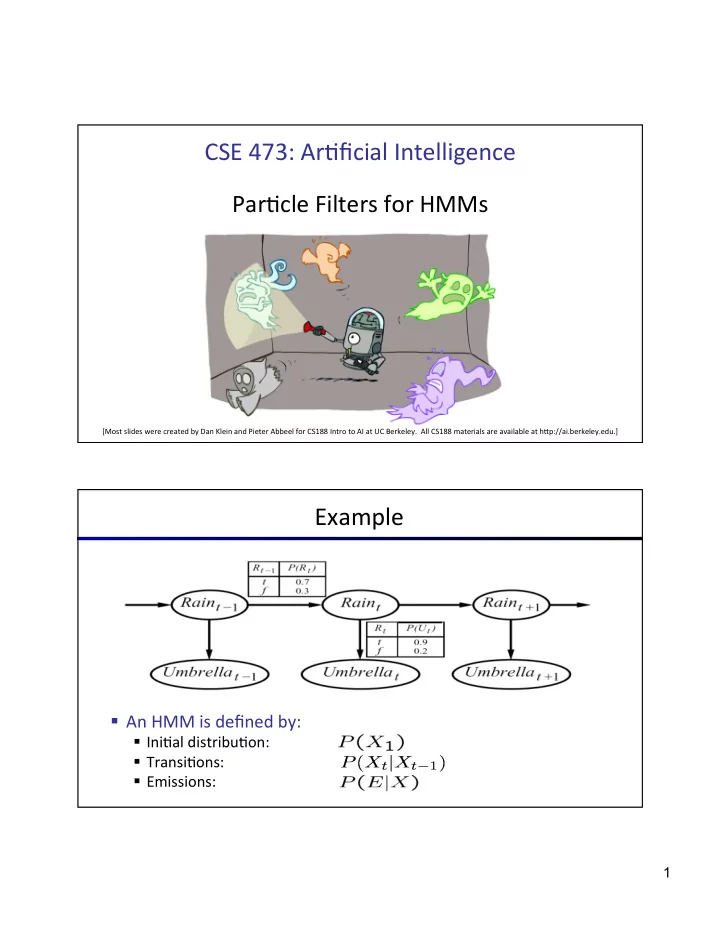
Elapse ¡ Weight ¡ Resample ¡

Par+cles: ¡ ¡ ¡ ¡ ¡(3,2) ¡ ¡ ¡ ¡ ¡(2,3) ¡ ¡ ¡ ¡ ¡(3,2) ¡ ¡ ¡ ¡ ¡ ¡ ¡ ¡(3,1) ¡ ¡ ¡ ¡ ¡(3,3) ¡ ¡ ¡ ¡ ¡(3,2) ¡ ¡ ¡ ¡ ¡(1,3) ¡ ¡ ¡ ¡ ¡(2,3) ¡ ¡ ¡ ¡ ¡(3,2) ¡ ¡ ¡ ¡ ¡(2,2) ¡ ¡ ¡ ¡ ¡ ¡Par+cles: ¡ ¡ ¡ ¡ ¡(3,2) ¡ ¡w=.9 ¡ ¡ ¡ ¡ ¡(2,3) ¡ ¡w=.2 ¡ ¡ ¡ ¡ ¡(3,2) ¡ ¡w=.9 ¡ ¡ ¡ ¡ ¡(3,1) ¡ ¡w=.4 ¡ ¡ ¡ ¡ ¡(3,3) ¡ ¡w=.4 ¡ ¡ ¡ ¡ ¡(3,2) ¡ ¡w=.9 ¡ ¡ ¡ ¡ ¡(1,3) ¡ ¡w=.1 ¡ ¡ ¡ ¡ ¡(2,3) ¡ ¡w=.2 ¡ ¡ ¡ ¡ ¡(3,2) ¡ ¡w=.9 ¡ ¡ ¡ ¡ ¡(2,2) ¡ ¡w=.4 ¡ (New) ¡Par+cles: ¡ ¡ ¡ ¡ ¡(3,2) ¡ ¡ ¡ ¡ ¡(2,2) ¡ ¡ ¡ ¡ ¡(3,2) ¡ ¡ ¡ ¡ ¡ ¡ ¡ ¡(2,3) ¡ ¡ ¡ ¡ ¡(3,3) ¡ ¡ ¡ ¡ ¡(3,2) ¡ ¡ ¡ ¡ ¡(1,3) ¡ ¡ ¡ ¡ ¡(2,3) ¡ ¡ ¡ ¡ ¡(3,2) ¡ ¡ ¡ ¡ ¡(3,2) ¡

[Demos: ¡ghostbusters ¡par+cle ¡filtering ¡(L15D3,4,5)] ¡

14

Video ¡of ¡Demo ¡– ¡Moderate ¡Number ¡of ¡Par+cles ¡ Video ¡of ¡Demo ¡– ¡One ¡Par+cle ¡

15

Video ¡of ¡Demo ¡– ¡Huge ¡Number ¡of ¡Par+cles ¡ Robot ¡Localiza+on ¡

§ In ¡robot ¡localiza+on: ¡

§ We ¡know ¡the ¡map, ¡but ¡not ¡the ¡robot’s ¡posi+on ¡ § Observa+ons ¡may ¡be ¡vectors ¡of ¡range ¡finder ¡readings ¡ § State ¡space ¡and ¡readings ¡are ¡typically ¡con+nuous ¡(works ¡ basically ¡like ¡a ¡very ¡fine ¡grid) ¡and ¡so ¡we ¡cannot ¡store ¡B(X) ¡ § Par+cle ¡filtering ¡is ¡a ¡main ¡technique ¡ ¡

16

Par+cle ¡Filter ¡Localiza+on ¡(Sonar) ¡

[Video: ¡global-­‑sonar-­‑uw-­‑annotated.avi] ¡

Par+cle ¡Filter ¡Localiza+on ¡(Laser) ¡

[Video: ¡global-­‑floor.gif] ¡

17

Robot ¡Mapping ¡

§ SLAM: ¡Simultaneous ¡Localiza+on ¡And ¡Mapping ¡

§ We ¡do ¡not ¡know ¡the ¡map ¡or ¡our ¡loca+on ¡ § State ¡consists ¡of ¡posi+on ¡AND ¡map! ¡ § Main ¡techniques: ¡Kalman ¡filtering ¡(Gaussian ¡HMMs) ¡ and ¡par+cle ¡methods ¡

DP-­‑SLAM, ¡Ron ¡Parr ¡ [Demo: ¡PARTICLES-­‑SLAM-­‑mapping1-­‑new.avi] ¡

Par+cle ¡Filter ¡SLAM ¡– ¡Video ¡1 ¡

[Demo: ¡PARTICLES-­‑SLAM-­‑mapping1-­‑new.avi] ¡

18

Par+cle ¡Filter ¡SLAM ¡– ¡Video ¡2 ¡

[Demo: ¡PARTICLES-­‑SLAM-­‑fastslam.avi] ¡