Definitions and Examples I (10.1) Definitions and Examples I (10.1) - - PowerPoint PPT Presentation

definitions and examples i 10 1 definitions and examples
SMART_READER_LITE
LIVE PREVIEW

Definitions and Examples I (10.1) Definitions and Examples I (10.1) - - PowerPoint PPT Presentation

Outline: Chapter 10 Stochastic Processes 2 Definitions and Examples (10.1) D fi i i d E l (10 1) Types of Stochastic Processes (10.2) 204312 PROBABILITY AND 204312 PROBABILITY AND Random Variables from Random Processes RANDOM


slide-1
SLIDE 1

204312 PROBABILITY AND 204312 PROBABILITY AND RANDOM PROCESSES FOR COMPUTER ENGINEERS COMPUTER ENGINEERS

Lecture 12: Chapter 10 p

1st Semester, 2007 Monchai Sopitkamon, Ph.D.

Outline: Chapter 10 Stochastic Processes

D fi i i d E l (10 1)

2

Definitions and Examples (10.1) Types of Stochastic Processes (10.2) Random Variables from Random Processes

(10.3) ( 0 3)

Independent, Identically Distributed Random

Sequences (10 4) Sequences (10.4)

The Poisson Process (10.5) Properties of Poisson Process (10.6) Expected Value and Correlation (10.8)

p ( )

Definitions and Examples I (10.1) Definitions and Examples I (10.1)

Stochastic = random Process = function of time Stochastic process = random functions of time P

b th f f f t f

Prob theory focuses on frequency of an event from

an experiment.

Stochastic processes are concerned also with time

sequences of the events.

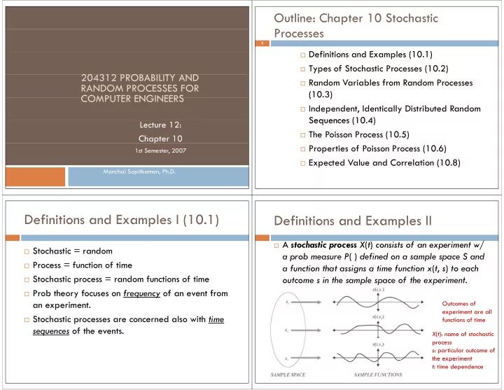
Definitions and Examples II Definitions and Examples II

A stochastic process X(t) consists of an experiment w/ A stochastic process X(t) consists of an experiment w/

a prob measure P( ) defined on a sample space S and a function that assigns a time function x(t s) to each a function that assigns a time function x(t, s) to each

  • utcome s in the sample space of the experiment.

Outcomes of experiment are all p functions of time X(t): name of stochastic process s: particular outcome of the experiment the experiment t: time dependence

slide-2
SLIDE 2

Definitions and Examples III Definitions and Examples III

Sample Function: A sample function x(t, s) is the time

function associated with outcome s of an experiment.

A sample function corresponds to an outcome of a

stochastic process experiment. p p

Ensemble: The ensemble of a stochastic process is the

set of all possible time functions that can result from set of all possible time functions that can result from an experiment.

Definitions and Examples IV Definitions and Examples IV

Ex.10.1: Starting at launch time t = 0, X(t) = temp

in °K on space shuttle’s surface. With each launch s, we record a temp sequence x(t, s). The ensemble of the experiment can be viewed as a group of the possible temp sequences. For example,

x(8073.68, 175) = 207 (8073 68, 75) 07 i th 175th l h

t s temp

174th 207

means in the 175th launch, the temp at t = 8073.68 sec

175th t = 8073.68

after this launch is 207°K

176th

Definitions and Examples V Definitions and Examples V

Since the stochastic process produces two-dimensional sample Since the stochastic process produces two-dimensional sample

functions, there are two types of averages

Ensemble average: taken at t = t0, X(t0) is a RV, and we have the

averages (expected value and variance) that we studied before averages (expected value and variance) that we studied before

Time average of a specific sample function: applied to a specific

sample function, x(t, s0), and gives a number for this sample function.

Ex.10.2: From Ex.10.1, over all possible launches (s), the avg temp

after 8073.68 sec is E(X(8073.68)) = 217°K (ensemble avg). In the 175th launch, the avg temp over that space shuttle mission is

671208.3

1 ( ,175) 187.43 671208.3 x t dt K = °

175th

where the integral limit 671208.3 is the duration in sec of the shuttle mission.

t

Time a erage Time average

Definitions and Examples VI Definitions and Examples VI

0 4 A h d M( ) h f

Ex.10.4: An experiment where we record M(t), the no of

active calls at a phone switch at time t, at each second

  • ver an interval of 15 min One trial of experiment
  • ver an interval of 15 min. One trial of experiment

yields sample fn m(t, s) shown in the fig. Each experiment performed yields some other fn m(t, s). This p p y ( , ) fn depends on the no of calls at the start of the

  • bservation period, the arrival times of new calls, and

the duration of each call. An ensemble average is the avg no of calls in progress at t = 403 sec. A time avg is the avg no of calls in progress during a certain 15 min the avg no of calls in progress during a certain 15-min interval.

slide-3
SLIDE 3

Definitions and Examples V Definitions and Examples V

Figure 10.2 (p. 356)

A sample function m(t,s) of the random process M(t) described in Example 10.4. p ( , ) p ( ) p

Definitions and Examples VI Definitions and Examples VI

RV h k l f i (t ) i l d

RVs that make up sample function m(t, s) include: m(0, s): the no of ongoing calls at the start of experiment X

X : the remaining time in sec of each of the m(0

X1, …, Xm(0, s): the remaining time in sec of each of the m(0,

s) ongoing calls

N: the no of new calls that arrive during the experiment S1, …, SN: the arrival times in sec of the N new calls Y1, …, YN: the calls durations in sec of each of the N new

calls calls

X1, . . . , XN : the interarrival times of the N new arrivals H, the number of calls that hang up during the experiment D1, . . . , DH: the call completion times of the H calls that

hang up

Types of Stochastic Processes I (10.2) Types of Stochastic Processes I (10.2)

Discrete-Value and Continuous-Value Processes X(t) is a discrete-value process if the set of all possible

values of X(t) at all times t is a countable set SX;

  • therwise X(t) is a continuous-value process.

Discrete-Time and Continuous-Time Processes X(t) is a discrete-time process if X(t) is defined only for

( ) p ( ) y a set of time instants; tn = nT, where T is a constant and n is an integer; otherwise X(t) is a continuous-time process.

Types of Stochastic Processes II Types of Stochastic Processes II

Brownian Motion Process P i P Poisson Process

Sample functions of four kinds of stochastic processes. Xcc(t) is a continuous-time, continuous-value process. Xdc(t) is discrete-time, continuous-value process obtained by sampling Xcc(t) every 0.1 seconds. Rounding Xcc(t) to the nearest integer yields Xcd(t), a continuous-time, discrete-value process. Lastly, Xdd(t), a discrete-time, discrete-value process, can be obtained either by sampling Xcd(t) or by rounding Xdc(t).

slide-4
SLIDE 4

Types of Stochastic Processes III Types of Stochastic Processes III

h f f d h

From the previous fig., for a discrete-time process, the

sample function is completely described by the ordered sequence of RVs X = X(nT) sequence of RVs Xn = X(nT).

Random Sequence A random sequence X is an ordered sequence of RVs X A random sequence Xn is an ordered sequence of RVs X0,

X1, …

Quiz10.2: For the temperature measurements of Quiz10.2: For the temperature measurements of

Ex.10.3, construct examples of the measurement process such that the process is either

a)

Discrete-time, discrete-value

b)

Discrete-time, continuous-value

c)

Continuous-time, discrete-value

d)

Continuous-time, continuous-value

Types of Stochastic Processes IV Types of Stochastic Processes IV

14

W b l d

a)

We obtain a continuous time, continuous valued process when we record the temperature as a continuous waveform over time continuous waveform over time

b)

If at every moment in time, we round the temperature to the nearest degree then we obtain a continuous to the nearest degree, then we obtain a continuous time, discrete valued process

c)

If we sample the process in part (a) every T seconds

c)

If we sample the process in part (a) every T seconds, then we obtain a discrete time, continuous valued process

d)

Rounding the samples in part (c) to the nearest integer degree yields a discrete time, discrete valued process.

Random Variables from Random Processes I (10.3)

We use X(t1) to represent a RV whose sample value

is x(t1, s), which is a sample fn x(t, s) at particular time instant t1 and sequence s.

However, X(t) can refer to either the random process

, ( ) p

  • r the RV that corresponds to the value of the

random process at time t. random process at time t.

If X(t1) is a discrete RV, it has a PMF

If X( ) i i RV i h PDF

1

( )( ) X t

P x ( ) f

If X(t1) is a continuous RV, it has a PDF

1

( )( ) X t

f x

Random Variables from Random Processes II

0 8 S 2

Ex.10.8: Suppose that at time instants T = 0, 1, 2,

…, we roll a die and record the outcome NT where 1 ≤ N ≤ 6 W th d fi th d 1 ≤ NT ≤ 6. We then define the random process X(t) such that for T ≤ t ≤ T + 1, X(t) = NT. In this case the experiment consists of an infinite sequence case, the experiment consists of an infinite sequence

  • f rolls and a sample fn is just the waveform

corresponding to the particular sequence of rolls corresponding to the particular sequence of rolls. What is the PMF of X(3.5)?

The RV X(3.5) is the value of the die roll at time 3. The RV X(3.5) is the value of the die roll at time 3.

(3.5)

1/ 6 1,...,6, ( ) th i

X

x P x = ⎧ = ⎨ ⎩ = prob that X = x (x = 1, …, 6) at time t = 3

(3.5)

  • therwise

(3.5)( ) X

P x

slide-5
SLIDE 5

Random Variables from Random Processes III

Ex.10.9: Let X(t) = R|cos2πft| be a rectified cosine signal

having a random amplitude R with the exponential PDF

1 ⎧

/10

1 0, 10 ( )

  • therwise

r R

e r f r

⎧ ≥ ⎪ ⎪ = ⎨ ⎪

What is the PDF fX(t)(x)?

  • therwise.

⎪ ⎪ ⎩

Since X(t) ≥ 0 for all t, P(X(t) ≤ x) = 0 for all x < 0. If x ≥ 0, and cos2πft > 0, P(X(t) ≤ x) = P(R ≤ x/|cos2πft|)

/ 2 f / cos2

( )

x ft R

f r dr

π

= ∫

/ 2 1 ft

/ cos2 /10 /10

/ cos2 1 10

x ft r r

x ft e dr e

π

π

− −

= = −

∫ Random Variables from Random Processes IV

/

= − e-x/10|cos2πft| − (−1) = 1 − e-x/10|cos2πft| When cos2πft ≠ 0, the complete CDF of X(t) is

x ⎧ < ⎪

( ) /10 cos2

0, ( ) 1 0.

X t x ft

x F x e x

π −

⎧ < ⎪ = ⎨ − ≥ ⎪ ⎩

When cos2πft ≠ 0, the PDF of X(t) is

/10 cos2

1

x ft π −

⎧ ≥ ⎪

/10 cos2 ( ) ( )

0, 10 cos2 ( ) ( ) th i

x ft X t X t

e x ft d F x f x dx

π

π ⎧ ≥ ⎪ ⎪ = = ⎨ ⎪0

  • therwise.

⎪ ⎪ ⎩

Random Variables from Random Processes V

19

Q i 10 3 I d ti li f 1K Ω i t th t l

Quiz 10.3: In a production line for 1K Ω resistors, the actual

resistance in ohms of each resistor is a uniform (950, 1050) RV R. The resistances of different resistors are independent. / The resistor company has an order for 1% resistors w/ a resistance between 990 – 1010 Ω. An automatic tester takes one resister /sec to measure its exact resistance. The / random process N(t) denotes the no of 1% resistors found in t sec. The RV Tr sec is the elapsed time at which r 1% resistors are found. resistors are found.

1.

What is p: the prob that any single resistor is a 1% resistor?

2.

What is the PMF of N(t)?

3.

What is E(T1) sec, the expected time to find the first 1% resistors?

4.

What is the prob that the first 1% resistor is found in exactly 5 p y sec?

Random Variables from Random Processes VI

20

E h i t h i t R i h ith if PDF

1.

Each resistor has resistance R in ohms with uniform PDF

0.01 950 1050, ( ) th i

R

r f r ≤ ≤ ⎧ = ⎨ ⎩

The prob that a test produces a 1% resistor is p = P(990 ≤ R ≤ 1010) = = 0 2

( )

  • therwise.

R

f ⎨ ⎩

( )

1010 0 01 dr

p = P(990 ≤ R ≤ 1010) = = 0.2

2

In t seconds, exactly t resistors are tested. Each resistor is a

( )

990

0.01 dr

2.

In t seconds, exactly t resistors are tested. Each resistor is a 1% resistor with probability p, independent of any other

  • resistor. Consequently, the number of 1% resistors found

has the binomial PMF has the binomial PMF

( ) ( )

0.2 0.8 0,1,..., ( ) 1

t n n t n n

t n t n t P

− −

⎧⎛ ⎞ = ⎪⎜ ⎟ ⎛ ⎞ ⎪⎝ ⎠ ⎨ ⎜ ⎟

( )

( )( )

1

  • therwise.

n N t

P n p p n = − = ⎨ ⎜ ⎟ ⎝ ⎠ ⎪ ⎪ ⎩

slide-6
SLIDE 6

Random Variables from Random Processes VII

21

f M f

3.

First we will find the PMF of T1. This problem is easy if we view each resistor test as an ind trial. A t i l ith b bilit if success occurs on a trial with probability p if we find a1% resistor. The first 1% resistor is found at time T = t if we observe failures on trials 1 time T1 = t if we observe failures on trials 1, . . . , t − 1 followed by a success on trial t. Hence, T1 has the geometric PMF the geometric PMF

( ) ( )

1

1 1

0.8 0.2 0,1,2,... ( ) 1

  • therwise

t t T

t P t p p

− −

⎧ = ⎪ = − = ⎨ ⎪ ⎩

A geometric random variable with success probability p has expected value 1/p In this problem E(T ) = 1/p =

  • therwise.

⎪ ⎩

has expected value 1/p. In this problem, E(T1) = 1/p = 1/0.2 = 5 sec.

Random Variables from Random Processes VIII

22

4.

Since p = 0.2, the probability the first 1% resistor is found in exactly five seconds is

= (0.8)4(0.2) = 0.08192.

1 (5)

T

P

Independent, Identically Distributed (iid) Random Sequences I (10.4)

An iid random sequence is a random sequence Xn in

which … X-2, X-1, X0, X1, X2, … are iid RVs.

Theorem 10.1: Let Xn denote an iid random

  • sequence. For a discrete-value process, the sample

q p , p vector X = has joint PMF

( ) ( ) ( ) ( ) ( )

k

P x P x P x P x P x

1 k

n n

X X ′ ⎡ ⎤ ⎣ ⎦

  • For a continuous-value process, the joint PDF of X =

1 2 1

( ) ( ) ( ) ( ) ( )

X X X k X i i

P x P x P x P x P x

=

= =∏

  • X

p , j

is

k

1 k

n n

X X ′ ⎡ ⎤ ⎣ ⎦

  • 1

2 1

( ) ( ) ( ) ( ) ( )

X X X k X i i

f x f x f x f x f x

=

= =∏

  • X

Independent, Identically Distributed (iid) Random Sequences II

B lli P A B lli ( ) X i iid

Bernoulli Process: A Bernoulli (p) process Xn is an iid

random sequence in which each Xn is a Bernoulli (p) RV.

Ex 10 12: In a common model for communications the Ex.10.12: In a common model for communications, the

  • utput X1, X2, … of a binary source is modeled as a

Bernoulli (p = ½) process.

Ex.10.13: Each day we buy a ticket for the NY Pick 4

  • lottery. Xn = 1 if our ticket on day n is a winner;
  • therwise X = 0 The random sequence X is a
  • therwise, Xn = 0. The random sequence Xn is a

Bernoulli process.

Ex.10.14: For the resistor process in Quiz 10.3, let Yn =

p ,

n

1 if, in the nth sec, we find a 1% resistor; otherwise Yn =

  • 0. The random sequence Yn is a Bernoulli process.
slide-7
SLIDE 7

Independent, Identically Distributed (iid) Random Sequences III

Ex.10.15: For a Bernoulli (p) process Xn, find the joint PMF

  • f X = [

]

1 n

X X ′

  • For a single sample Xi, we can write the Bernoulli PMF in

the following way: ( ) { }

1

1 0,1 , ( )

i i

x x i

p p x P

⎧ − ∈ ⎪ ⎨

When xi ∈ {0, 1} for i = 1, …, n, the joint PMF can be ( ) { }

( )

  • therwise.

i

i X i

p p P x ⎪ = ⎨ ⎪ ⎩

When xi ∈ {0, 1} for i 1, …, n, the joint PMF can be written as

( ) ( )

1 1

( ) 1 1

i i

n x n k x k i

P x p p p p

− − =

= − = −

X

( )

( )

{ }

1 1

1 0 1 1

n n

n x x x x

p p x i n

− + + + +

⎧ − ∈ = ⎪

  • where k = x1 + … + xn. The complete expression for the

joint PMF is

1 i=

( ) { }

1 0,1 , 1,..., ( )

  • therwise.

i

p p x i n P x ⎧ − ∈ = ⎪ = ⎨ ⎪ ⎩

X

Independent, Identically Distributed (iid) Random Sequences IV

Quiz 10.4: For an iid random sequence Xn of

Gaussian(0, 1) RVs, find the joint PDF of X =

Since each Xi is a N(0, 1) random variable, each Xi has

[ ]

1 m

X X ′

  • Since each Xi is a N(0, 1) random variable, each Xi has

PDF

2 /2

( )

1 ( ) 2

x X i

f x e π

= By Theorem 10.1, the joint PDF of X = is 2π

[ ]

1 m

X X ′

  • (

) ( ) ( )

2 2 1

( )/2 (1),..., ( ) 1 /2 1

1 ( ) ,..., 2

m

m x x X X m m X i m i

f x f x x f x e π

− + + =

= = =

  • X

( )

The Poisson Process I (10.5) The Poisson Process I (10.5)

Counting Process: A stochastic process N(t) is a

counting process if for every sample function, n(t, s) = 0 for t < 0 and n(t, s) is integer-valued and nondecreasing with time.

N(t) = no of arrivals at a system during interval (0, t]. Each jump in the fig Each jump in the fig.

represents one arrival.

The no of arrivals

during interval (t0, t1] = N(t1) – N(t0)

The Poisson Process II The Poisson Process II

N(t) is Poisson RV with PMF: N(t) is Poisson RV with PMF:

( )

( )

/ ! 0,1,2, , ( ) th i

n T N T

T e n n P n

λ

λ

⎧ = ⎪ = ⎨ ⎪ …

For any interval (t0, t1], the no of arrivals has a Poisson PMF w/ parameter λT where T = t – t

  • therwise.

⎪ ⎩

w/ parameter λT where T = t1 – t0.

Poisson Process: A counting process N(t) is a Poisson process of

rate λ if

1.

The no of arrivals in any interval (t0, t1], N(t1) – N(t0), is a Poisson RV w/ expected value λ(t1 – t0)

2.

For any pair of nonoverlapping intervals (t0, t1] and (t0

′, t1 ′], the 2.

For any pair of nonoverlapping intervals (t0, t1] and (t0 , t1 ], the no of arrivals in each interval, N(t1) – N(t0) and N(t1

′) – N(t0 ′)

respectively, are independent RVs.

  • λ = arrival rate of the Poisson process
  • λ = arrival rate of the Poisson process
  • Expected no of arrivals per unit time = E(N(t))/t = λ
slide-8
SLIDE 8

The Poisson Process III The Poisson Process III

M = N(t ) N(t ) has PMF M = N(t1) – N(t0) has PMF

( )

( )

( )

1

1

0,1,..., !

m t t

t t e m

λ

λ

− −

⎧ − ⎪ = ⎪ ! ( )

  • therwise.

M

m P m ⎪ = ⎨ ⎪ ⎪ ⎩

For a Poisson process N(t) of rate λ, the joint PMF of N

= for ordered time instants t1 < … <

( ) ( )

1 ,

,

k

N t N t ′ ⎡ ⎤ ⎣ ⎦ …

for ordered time instants t1 … tk is ( ) ( )

1 ,

,

k

N t N t ⎡ ⎤ ⎣ ⎦ … ( ) ( )

1 1 1 2 1 2

1 2 1

, ! ! !

k k k

n n n n n k k k k

e e e n n n n n n n

α α α

α α α

− − − − −

⎧ ≤ ≤ ≤ ⎪ − − ⎪

  • (

) ( )

1 2 1 1

! ! ! ( )

  • therwise.

k k

n n n n n P n

⎪ = ⎨ ⎪ ⎪ ⎩

N

where α1 = λt1, and for i = 2, …, k, αi = λ(t1 – ti-1).

The Poisson Process IV The Poisson Process IV

For a Poisson process of rate λ, the interarrival times

/ X1, X2,… are an iid random sequence w/ the exponential PDF

λ

⎧ 0, ( )

  • therwise.

x X

e x f x

λ

λ

⎧ ≥ = ⎨ ⎩

A counting process w/ ind exponential (λ) interarrivals

X X i P i f t λ ⎩ X1, X2,… is a Poisson process of rate λ.

The Poisson Process V The Poisson Process V

Q i 10 5 D t k t t itt d b d

Quiz 10.5: Data packets transmitted by a modem over

a phone line form a Poisson process of rate 10 packets/sec Using M to denote the no of packets packets/sec. Using Mk to denote the no of packets transmitted in the kth hour, find the joint PMF of M1 and M2. The first and second hours are nonoverlapping i t l Si h l 3600 d th

  • intervals. Since one hour equals 3600 sec and the

Poisson process has a rate of 10 packets/sec, the expected number of packets in each hour is E(M) = λt expected number of packets in each hour is E(Mi) = λt = 10*3600 = 36,000 = α. This implies M1 and M2 are independent Poisson random variables each with PMF independent Poisson random variables each with PMF

The Poisson Process VI The Poisson Process VI

32

m α −

⎧ 0,1,2,... ! ( )

i

m M

e m m P m

α

α ⎧ = ⎪ ⎪ = ⎨ ⎪

Since M1 and M2 are independent the joint PMF of M1 and

  • therwise

⎪ ⎪ ⎩

Since M1 and M2 are independent, the joint PMF of M1 and M2 is

1 1

2

0 1 2 ;

m m

m e

α

α

+ −

= ⎧

1 1 1 2 1

1 2 1 2 , 1 2 1 2 2

0,1,2,...; 0,1,2,..., ! ! ( , ) ( ) ( )

M M M M

m e m m m P m m P m P m α = ⎧ ⎪ = ⎪ = = ⎨ ⎪

1 2 1

  • therwise

⎪ ⎪ ⎩

slide-9
SLIDE 9

Properties of the Poisson Process I (10.6)

33

M l P t Memoryless Property:

( , ) ( | )

x n n

P X t x X t P X t x X t e λ

> + > > + > = = If the arrival has not occurred by time t, the additional time ( | ) ( )

n n n

P X t x X t e P X t > + > > y , until the arrival, Xn – t, has the same exponential distribution as Xn.

Xn Xn-1 Xn+1

No matter how long we have waited for the arrival, the i i i il h i l i

t x

remaining time until the next arrival remains an exponential (λ) RV.

Properties of the Poisson Process II Properties of the Poisson Process II

34

Let N1(t) and N2(t) be two independent Poisson

processes of rates λ1 and λ2. The counting process N(t) = N1(t) + N2(t) is a Poisson process of rate λ1 + λ2.

( )

1 2

1 2 1 2

1 0, ( ) ( , ) ( ) ( ) 0.

x

x P X x P X x X x P X x P X x e x

λ λ − +

⎧ < ⎪ > = > > = > > = ⎨ ≥ ⎪ ⎩ ⎪ ⎩

Properties of the Poisson Process III Properties of the Poisson Process III

35

Ex.10.16: Cars, trucks, and buses arrive at a toll

booth as ind Poisson processes w/ rates λc =1.2, λt = 0.9, and λb = 0.7 per min, respectively. In a 10- min interval, what is the PMF of N, the no of vehicles (cars, trucks, or buses) that arrive? By previous eq., the arrival of vehicles is a By previous eq., the arrival of vehicles is a Poisson process of rate λ = 1.2 + 0.9 + 0.7 = 2.8 vehicle/min. In a 10-min interval, λt = 2.8 x 10 = vehicle/min. In a 10 min interval, λt 2.8 x 10 28, and N has PMF

( )

28

28 / ! 0,1,2, ,

n n t

e n n

λ −

⎧ = …

( )

28 / ! 0,1,2, , ( ) / !

  • therwise.

n t N

e n n P n t e n

λ

λ

⎧ = = ⎨ ⎩ …

Properties of the Poisson Process IV Properties of the Poisson Process IV

36

Bernoulli Decomposition: Divide a Poisson process into two separate processes: Type I

and Type II processes

The types I and II arrivals have prob p and (1 – p),

respectively

The counting processes N1(t) and N2(t) derived from a

Bernoulli decomposition of the Poisson process N(t) are ind Poisson processes w/ rates λp and λ(1 – p).

Interpretation: Two ind Poisson processes N1(t) and N2(t) w/

rates λ1 and λ2 can be constructed from a Bernoulli decomposition of a Poisson process N (t) w/ rate λ1+λ2 by choosing the success prob to be p = λ1/(λ1+λ2).

slide-10
SLIDE 10

Properties of the Poisson Process V Properties of the Poisson Process V

37

E 10 17 A W b d hit P i t

Ex.10.17: A Web server records hits as a Poisson process at

a rate of 10 hits/s. Each page is either an internal request w/ prob 0.7 from the intranet or an external request w/ prob 0.3 from the Internet. Over a 10-min interval, what is the PMF of I, the no of internal requests, and X, the no of external requests? q

Internal requests has Poisson process w/ rate (λ) 10x0.7=7 hits/s and parameter αI = 7x10x60=4200 hits. External requests has Poisson process w/ rate (λ) 10x0 3=3 hits/s External requests has Poisson process w/ rate (λ) 10x0.3=3 hits/s and parameter αX = 3x10x60=1800 hits. Both types of requests are independent Poisson processes. M f The joint PMF of I and X is:

{ }

4200 1800

4200 1800 , 0,1, , ! !

i x

e e i x i x

− −

⎧ ∈ ⎪ ⎪ …

.

,

! ! ( , ) ( ) ( )

  • therwise.

I X I X

i x P i x P i P x ⎪ = = ⎨ ⎪ ⎪ ⎩

Expected Value and Correlation I (10.8)

38

For a stochastic process X(t), X(t1), the value of a

sample function at time instant t1 is a RV.

Therefore, X(t1) has a PDF

and expected value .

( ) ( )

1

X t

f x ( )

( )

1

E X t

The expected value of a stochastic process X(t) is

the deterministic function (since the value of

( )

( )

1

( )

( )

E X t

the deterministic function (since the value of is just a number) ( ) E(X( ))

( )

( )

1

E X t

μX(t) = E(X(t))

Expected Value and Correlation II Expected Value and Correlation II

E 10 18 If R i i RV fi d h d

Ex.10.18: If R is a nonnegative RV, find the expected

value of X(t) = R|cos2πft|.

X(t) has expected value X(t) has expected value

μX(t) = E(X(t)) = E(R|cos2πft|) = E(R)|cos2πft|

Autocovariance:

u oco a a ce:

From Cov(X, Y) indicates how much info RV X tells about RV

Y. Hi h l f C () id hi h di bili f l f

High value of Cov() provides high predictability of value of

Y from observing value of X.

Autocovariance measures how much the two RVs X(t1) and

( 1) X(t1+τ) of a sample fn X(t) taken at times t1 and t1+τ differ in the τ sec different between t1 and t1+τ.

The higher the autocovariance the less the change of X(t) in the τ The higher the autocovariance, the less the change of X(t) in the τ

sec interval

Near zero autocovariance indicates rapid change

Expected Value and Correlation III Expected Value and Correlation III

40

The autocovariance fn of the stochastic process X(t)

is CX(t, τ) = Cov(X(t), X(t + τ))

The autocovariance fn of the random sequence Xn is

CX(m, k) = Cov(X , X +k) CX(m, k) Cov(Xm, Xm+k)

The autocorrelation fn of the stochastic process X(t) is

R (t τ) = E(X(t)X(t + τ)) RX(t, τ) = E(X(t)X(t + τ))

The autocorrelation fn of the random sequence Xn is

RX(m, k) = E(XmXm+k)

slide-11
SLIDE 11

Expected Value and Correlation IV Expected Value and Correlation IV

41

l f f

The autocorrelation and autocovariance fns of a

process X(t) satisfy CX(t, τ) = RX(t, τ) – μX(t)μX(t+τ)

The autocorrelation and autocovariance fns of a

random sequence Xn satisfy CX(n, k) = RX(n, k) – μX(n)μX(n+k)

X X

μX μX

Note: Autocovariance is useful when we want to use

X(t) to predict a future value X(t + τ), whereas the ( ) p ( ), autocorrelation is used to describe the power of a random signal.