DEVELOPING ANISOTROPIC BEAM ELEMENT FOR DESIGN OF COMPOSITE WIND - - PDF document

SLIDE 1

18TH INTERNATIONAL CONFERENCE ON COMPOSITE MATERIALS

1 Introduction For wind turbines blades, composite materials are widely used because they can reduce the total weight while retaining the structural properties and because they have good tailoring and fatigue life

• characteristics. The tailoring capability of the

composite blade could be used to passively control the wind turbine response and results in a decrease

• f fatigue loads and the risk of flutter. However, the

aeroelastic codes in the wind energy fields such as HAWC2 still use the classical beam models. It cannot be used to investigate the coupling effects of anisotropic materials. It is shown in [1] that a typical wind turbine blade has very small couplings, but that these can be introduced easily by adding angled unidirectional layers. In this paper a new beam element which is able to consider anisotropic characteristics of a beam is developed and implemented into the structural part

• f the HAWC2.

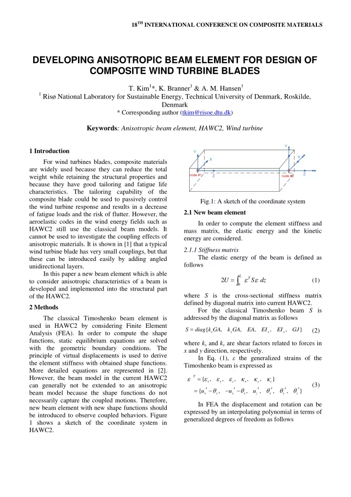
2 Methods The classical Timoshenko beam element is used in HAWC2 by considering Finite Element Analysis (FEA). In order to compute the shape functions, static equilibrium equations are solved with the geometric boundary conditions. The principle of virtual displacements is used to derive the element stiffness with obtained shape functions. More detailed equations are represented in [2]. However, the beam model in the current HAWC2 can generally not be extended to an anisotropic beam model because the shape functions do not necessarily capture the coupled motions. Therefore, new beam element with new shape functions should be introduced to observe coupled behaviors. Figure 1 shows a sketch of the coordinate system in HAWC2. Fig.1: A sketch of the coordinate system 2.1 New beam element In order to compute the element stiffness and mass matrix, the elastic energy and the kinetic energy are considered. 2.1.1 Stiffness matrix The elastic energy of the beam is defined as follows 2

L T

U S dz (1) where S is the cross-sectional stiffness matrix defined by diagonal matrix into current HAWC2. For the classical Timoshenko beam S is addressed by the diagonal matrix as follows

{ , , , , , }

x y x y

S diag k GA k GA EA EI EI GJ

(2) where kx and ky are shear factors related to forces in x and y direction, respectively. In Eq. (1), ε the generalized strains of the Timoshenko beam is expressed as

{ , , , , , } { , , , , , }

T x y z x y z x y y x z x y z

u u u

(3) In FEA the displacement and rotation can be expressed by an interpolating polynomial in terms of generalized degrees of freedom as follows

DEVELOPING ANISOTROPIC BEAM ELEMENT FOR DESIGN OF COMPOSITE WIND TURBINE BLADES

• T. Kim1*, K. Branner1 & A. M. Hansen1

1 Risø National Laboratory for Sustainable Energy, Technical University of Denmark, Roskilde,

Denmark

* Corresponding author (tkim@risoe.dtu.dk)

Keywords: Anisotropic beam element, HAWC2, Wind turbine

SLIDE 2

6 1 6 6

( ) { , , , , , } ( )

i i

T x y z x y z N N

q x u u u N x

(4) where N is the polynomial matrix in which,

2

1

n

N x x x

where n=1 for linear polynomial, α is the generalized degrees of freedom, and Ni is the highest power in the polynomial + 1. From the Eqs. (3) and (4) the generalized strain can be expanded in terms of strain-displacement matrix and generalized degrees of freedom as follows

6 1 6 6

( )

i i

N N

B x (5) where B is the strain-displacement matrix which includes polynomial matrix and its derivative terms as follows

1 6 6

( ) ( ) ( )

i

N

B x B N x B N x (6) By substituting Eq. (5) into Eq. (1), the elastic energy of the beam can be illustrated as follows 2

L T T D

U B SB dz (7) In order to find α in Eq. (7) the boundary conditions at the beam ends are satisfied and the beam sections are in equilibrium which can be

• btained when the total elastic energy is minimized.

By applying boundary conditions the nodal degrees

• f freedom are obtained as follows

1 1 2 12 1 6 1 2 12 6

i i

d N N

d N N N (8) Here N1 is a 12 by 12 matrix which is assumed to be invertible. Therefore, N1 and N2 become

1 2 2 3 12 12 12 6 12

,

i i

N N

I N N I LI L I L I L I

(9) where L is the length of the beam element. From Eq. (8) α1 can be rewritten as

1 1 1 2 2

N d N (10) Therefore α can be expressed as follows

1 2

1 1 1 1 1 2 2 2 12 (6 12) 12 12 1 2 6 1 12 1 (6 12) 1 (6 12) 12 (6 12) (6 12) 1 1 2 2 12 1 6 12 6 (6 12)

i i i i i i i i i

N N N N N N A A N N N

d N N N I I I A A

(6 12) 1 1 1 1 1 1 1 2 2 2 2

i

N

A N d A N N A

(11) To compute α vector, the total energy minimization approach in terms of

2 , 2

dU d

, is

• considered. From Eqs. (7) and (11), the total elastic

energy of the beam is obtained as follows

1 1 2 2 1 1 2 2 1 1 1 1 1 1 2 2 2 2

1 2

T

T T T T T T T T T

U d N A N N A A D A N d A N N A

(12) Resulting from the total energy minimization,

2 vector is obtained as follows 2 1 1 2 1 1 1 1 2 1 1 1 1 2 1 1 1 1 2 2 1 1 2 2 2 1 1 2 2 2 1 2 12 1 6 12 12 6 12 6 12

i i i

T T T T P T T T T T T T T Q N N N

dU d N N A DA N A DA N d N N A DA N N A DA N N N N A DA A DA Q P d

(13) By substituting Eq. (13) into Eq. (11), α vector as a function of the nodal degrees of freedom is represented as follows

1 1 1 1 1 1 1 1 2 2 1 1 1 1 1 1 1 1 2 2 6 12

i

N

A N d A N N Q Pd A Q Pd A N A N N Q P A Q P d N d (14)

SLIDE 3

3 DEVELOPING ANISOTROPIC BEAM ELEMENT FOR DESIGN OF COMPOSITE WIND TURINE BLADES

Finally, the elastic energy of the beam is

• btained in terms of nodal degrees of freedom by

substituting Eq. (14) into Eq. (7) as follows 1 2 1 2

L T T T T

U d N B SB dz N d d Kd (15) where K matrix, ,

L T T

K N B SB dz N is the element stiffness matrix. 2.1.2 Mass matrix The method to compute the element mass matrix is similar to the definition of the stiffness

• matrix. The element mass matrix is obtained from

the kinetic energy as follows 1 2 1 2

T V L T

T r rdV r Erdz (16) where

, ,

r , V and E are the mass density, velocity of

the body, volume of body and the cross-sectional mass matrix respectively. By applying the same shape function as the stiffness matrix, Eq. (16) can be extended as follows 1 ( ) ( ) 2 1 2

L T T T T

T d N N x EN x dz N d d Md (17) where M matrix, ,

L T T

M N N EN dz N is the element mass matrix. 3 Results After implementing this new beam element into HAWC2, three different cases are investigated in order to validate the new beam model. The effect

• f using anisotropic material is studied as well.

Three different cases are considered for this study. Figure 2 (a), (b), and (c) show a sketch of the considered cases. Table 1 shows the detailed structural properties and cross-sectional stiffness matrix for the first example. For Case 2 and Case 3,

• nly sectional stiffness information is displayed in

Table 2. More detailed information about the material properties and geometries are addressed in [3, 4]. (a) Case1: [0°]T layup with arbitrary isotropic material (b) Case2: [30°]T layup with Graphite/Epoxy (c) Case3: [45°/0°]3s layups with Graphite/Epoxy Fig.2: A sketch of considered cases Table1: Structural properties of Case 1 Material Arbitrary material E11, E22, E33 100 psi G12, G13, G23 41.6667 psi ν12, ν13, ν23 0.2 ρ 1 lb-sec2/in4 Width 0.1 in Height 0.1 in Length 7.5 in

SLIDE 4

Sectional stiffness from VABS S11, S22 3.4899×10-1 (lb) S33 1 (lb) S44, S55 8.3384×10-4 (lb-in2) S66 5.9084×10-4 (lb-in2) Table2: Sectional stiffness of Case 2 and 3 Stiffness of Case 2 [3] Stiffness of Case 3 [4] S11 0.1005×106 (lb) S11 0.9369×105 (lb) S13 0.1274×106 (lb) S13

• 0.4655×105 (lb)

S22 0.8634×104 (lb) S22 0.6798×104 (lb) S33 0.3566×106 (lb) S33 0.8116×106 (lb) S44 0.4578×103(lb-in2) S44 0.1852×103(lb-in2) S46

• 0.321×103(lb-in2)

S46 0.3448×102(lb-in2) S55 0.4062×104(lb-in2) S55 0.9179×105(lb-in2) S66 0.5069×103(lb-in2) S66 0.1249×103(lb-in2) Case 1 is used for validating whether the new beam model is correctly implemented into HAWC2

• r not. The other two cases are used for the

comparisons between new HAWC2 computation with anisotropic material and the other existing results obtained from [3, 4]. To compute sectional properties, VABS is used for Case 1. The other properties are directly imported from the references. 3.1 Validations Eigenvalue analysis is performed for the three different cases. Table 3 shows the natural frequency comparisons of Case 1 between new beam element before implementing HAWC2 and after

• implementation. They are completley identical.

From this result, it may be concluded that the new beam element is successfully implemented into HAWC2. Table 3: Natural frequency comparison of Case 1 Mode New beam element only [Hz] HAWC2 [Hz] 1 2.87262E-03 2.87262E-03 2 2.87262E-03 2.87262E-03 3 1.80466E-02 1.80466E-02 4 1.80466E-02 1.80466E-02 5 5.09409E-02 5.09409E-02 6 5.09409E-02 5.09409E-02 7 1.14752E-01 1.14752E-01 Table 4 shows the natural frequency comparisons between the other existing results and HAWC2

• computation. The HAWC2 result shows good

agreement with [3, 4], respectively. Table 4: Natural frequency comparisons of Case 2 and 3 Case 2 (Wenbin Yu et al.) Mode HAWC2 [Hz]

• Ref. [3] [Hz]

1 52.6 52.6 2 209.8 209.8 3 326.3 326.3 4 899.8 899.8 5 1284.9 1284.9 6 1661.8 1661.3 Case 3 (Hodges et al.) Mode HAWC2 [Hz] Ref.[4] [Hz] 1 4.66 4.66 2 29.17 29.60 3 81.53 84.89 4 113.36 113.43 where small discrepancies might occur due to using different shape functions. 3.2 Static deflection A static analysis is performed with Case 2 and 3 in order to investigate important physical differences between isotropic and anisotropic structures by using old versions (i.e. before implementing the new beam model) and new versions (i.e. after implementing the new beam model) of HAWC2. The old version of HACW2 considers the anisotropic characteristics produced by the shear center offset only [2, 5]. However, its effect is ignored in this paper. Thus, it is assumed that the shear center is located at the center of the considered sections for both cases. A cantilevered graphite-epoxy beam is

• considered. Figure 3 shows a sketch of the

cantilevered beam with static load and torsion. For the Case 2, 7.5in length of the beam and 1lb static load is applied. For the Case 3, 22.06in length and 1in-lb static torsion is applied.

SLIDE 5

5 DEVELOPING ANISOTROPIC BEAM ELEMENT FOR DESIGN OF COMPOSITE WIND TURINE BLADES

Fig.3: A sketch of the cantilevered graphite-epoxy beam The static deflections and rotations of Case 2 are presented in Fig. 4. In the figure, the blue and red colors represent anisotropic and isotropic results,

• respectively. From Table 2 it can be expected that

flapwise bending-torsion and axial-edgewise deflection are coupled on the structure. Therefore, when the static load is applied to the flapwise direction it should be produced that not only additional flapwise deflection but also additional flapwise bending which also results in torsion. From the results, the expected characteristics are observed with the new beam element while the isotropic model cannot capture the effects. Fig.4: Differences of the displacements between anisotropic and isotropic properties for Case 2 Figure 5 shows a comparison of the static deflections and rotations of Case 3. This case has the same couplings as Case 2. Therefore, when the torsion is applied to the structure, not only additional torsion but also additional flapwise bending which also results in flapwise deflection should be captured. From the results the new beam element captures the expected physical behavior correctly while the isotropic model does not. Fig.5: Differences of the displacements between anisotropic and isotropic properties for Case 3 Table 5 shows the natural frequency differences between the isotropic and the anisotropic

• model. The differences are obvious on the coupled

modes because the isotropic model does not have the abilities to capture the coupling effects between modes. Table5: Natural frequency differences between isotropic and anisotropic model HAWC2 simulation of Case 2 Mode Anisotropic [Hz] Isotropic [Hz]

SLIDE 6

1(flap) 52.6 70.6 2(edge) 209.8 210.1 3(flap) 326.3 436.4 4(flap) 899.8 1197.6 5(edge) 1284.9 1297.3 6(flap) 1661.8 2284.8 HAWC2 simulation of Case 3 Mode Anisotropic [Hz] Isotropic [Hz] 1 4.66 4.78 2 29.17 29.95 3 81.53 83.77 4 113.36 113.33 As we have investigated above there are big differences between isotropic and anisotropic results for both the static deflections and the natural

• frequencies. Both are very important parameters

when designing wind turbines. In that sense, the anisotropic behavior should be included in the relevant aeroelastic numerical tool if the blades have structural couplings. 4 Conclusion In this paper, the new beam element which is able to consider the anisotropic behaviors is developed and implemented into HAWC2. Validations for the beam model and implementation are performed with 3 different cases. The static analysis and eigenvalue analysis are performed. From the results it can be concluded that the anisotropic characteristics should be taken into account in order to obtain accurate results. Acknowledgment The work is partly supported by the Danish Energy Authority through the 2007 Energy Research Programme (EFP 2007). The supported EFP-project is titled “Anisotropic beam model for analysis and design of passive controlled wind turbine blades” and has journal no. 33033-0075. The support is gratefully acknowledged and highly appreciated. References

[1] Luczak, M., Manzato, S., Peeters, B., Branner, K., Berring, P. & Kahsin, M., “Dynamic Investigation of Twist-bend Coupling in a Wind Turbine Blade”, Journal of Theoretical and Applied Mechanics, Volume 49 Issue 3, 2011. [2] J.T. Petersen, “Kinematically Nonlinear Finite Element Model of a Horizontal Axis Wind Turbine- Part 1: Mathematical Model and Results,” Ph.D. Thesis, Technical University of Denmark, July, 1990 [3] W. Yu, “Efficient High-Fidelity Simulation of Multi- body Systems with Composite Dimensionally Reducible Components,” Journal of the American Helicopter Society, Vol. 52, no. 1, 2007, pp. 49-57. [4] D.H., Hodges, Nonlinear Composite Beam Theory, AIAA, Reston, VA, 2006. [5] T.J., Larsen and A.M., Hansen, “How 2 HAWC2, the user’s manual,” Risø-R-1597(EN), Dec. 2007.