DIMACS Tutorial on Phylogenetic Trees and Rapidly Evolving Pathogens - - PowerPoint PPT Presentation

DIMACS Tutorial on Phylogenetic Trees and Rapidly Evolving Pathogens

Katherine St. John City University of New York 1

Thanks to the DIMACS Staff

• Linda Casals
• Walter Morris
• Nicole Clark

Katherine St. John City University of New York 2

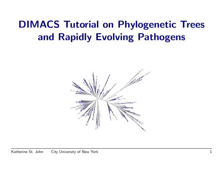
Tutorial Outline

• Day 1: Introduction to Phylogenetic Reconstruction
• Day 2: Applications to Rapidly Evolving Pathogens

Katherine St. John City University of New York 3

Tutorial Outline

• Day 1: Introduction to Phylogenetic Reconstruction

– Overview: Katherine St. John, CUNY – Parsimony Reconstruction of Phylogenetic Trees: Trevor Bruen, McGill University – Using Maximum Likelihood for Phylogenetic Tree Reconstruction: Rachel Bevan, McGill University – Hands-on Session: Constructing Trees Katherine St. John

• Day 2: Applications to Rapidly Evolving Pathogens

Katherine St. John City University of New York 4

Tutorial Outline

• Day 1: Intro to Phylogenetic Reconstruction
• Day 2: Applications to Rapidly Evolving Pathogens

– Statistical Overview: Alexei Drummond, University of Auckland – Tricks for trees: Having reconstructed trees, what can we do with them? Mike Steel, University of Canterbury – Hands-on Session: Katherine St. John

Katherine St. John City University of New York 5

Overview Outline

• Overview

Overview Outline

• Overview
• Constructing Trees

Overview Outline

• Overview
• Constructing Trees
• Constructing Networks

Overview Outline

• Overview
• Constructing Trees
• Constructing Networks
• Comparing Reconstruction Methods

Overview Outline

• Overview
• Constructing Trees
• Constructing Networks
• Comparing Reconstruction Methods
• Evaluating the Results

Katherine St. John City University of New York 6

Talk Outline

• Overview
• Constructing Trees
• Constructing Networks
• Comparing Reconstruction Methods
• Evaluating the Results

Katherine St. John City University of New York 7

Goal: Reconstruct the Evolutionary History

(www.amnh.org/education/teacherguides/dinosaurs)

Goal: Reconstruct the Evolutionary History

(www.amnh.org/education/teacherguides/dinosaurs)

The evolutionary process not only determines relationships among taxa, but allows prediction of structural, physiological, and biochemical properties.

Katherine St. John City University of New York 8

Process for Reconstruction: Input Data

Start with information about the taxa. For example: Morphological Characters

Process for Reconstruction: Input Data

Start with information about the taxa. For example: Morphological Characters Biomolecular Sequences

A

• GTTAGAAGGCGGCCAGCGAC. . .

B

• CATTTGTCCTAACTTGACGG. . .

C

• CAAGAGGCCACTGCAGAATC. . .

D

• CCGACTTCCAACCTCATGCG. . .

E

• ATGGGGCACGATGGATATCG. . .

F

• TACAAATACGCGCAAGTTCG. . .

(Other: molecular markers (ie SNPs), gene order, etc.)

Katherine St. John City University of New York 9

Process for Reconstruction

Process for Reconstruction

Input Data

A

• GTTAGAAGGC. . .

B

• CATTTGTCCT. . .

C

• CAAGAGGCCA. . .

D

• CCGACTTCCA. . .

E

• ATGGGGCACG. . .

F

• TACAAATACG. . .

Process for Reconstruction

Input Data

A

• GTTAGAAGGC. . .

B

• CATTTGTCCT. . .

C

• CAAGAGGCCA. . .

D

• CCGACTTCCA. . .

E

• ATGGGGCACG. . .

F

• TACAAATACG. . .

→ Reconstruction Algorithms

Maximum Parsimony Maximum Likelihood Distance Methods: NJ, Quartet-Based, Fast Convering, . . .

Process for Reconstruction

Input Data

A

• GTTAGAAGGC. . .

B

• CATTTGTCCT. . .

C

• CAAGAGGCCA. . .

D

• CCGACTTCCA. . .

E

• ATGGGGCACG. . .

F

• TACAAATACG. . .

→ Reconstruction Algorithms

Maximum Parsimony Maximum Likelihood Distance Methods: NJ, Quartet-Based, Fast Convering, . . .

→ Output Tree

Katherine St. John City University of New York 10

Applications

In addition to finding the evolutionary history of species, phylogeny is also used for:

Applications

In addition to finding the evolutionary history of species, phylogeny is also used for:

• drug discovery: used to determine structural and

biochemical properties of potential drugs

Applications

In addition to finding the evolutionary history of species, phylogeny is also used for:

• drug discovery: used to determine structural and

biochemical properties of potential drugs

• multiple sequence alignment

Applications

In addition to finding the evolutionary history of species, phylogeny is also used for:

• drug discovery: used to determine structural and

biochemical properties of potential drugs

• multiple sequence alignment
• origin of virus and bacteria strains

Katherine St. John City University of New York 11

Talk Outline

• Overview
• Constructing Trees
• Constructing Networks
• Comparing Reconstruction Methods
• Evaluating the Results

Katherine St. John City University of New York 12

Process for Reconstruction

Input Data

A

• GTTAGAAGGC. . .

B

• CATTTGTCCT. . .

C

• CAAGAGGCCA. . .

D

• CCGACTTCCA. . .

E

• ATGGGGCACG. . .

F

• TACAAATACG. . .

→ Reconstruction Algorithms

Maximum Parsimony Maximum Likelihood Distance Methods: NJ, Quartet-Based, Fast Convering, . . .

→ Output Tree

Katherine St. John City University of New York 13

Algorithms for Reconstruction

• Most optimization criteria are hard:

Algorithms for Reconstruction

• Most optimization criteria are hard:

– Maximum Parsimony: (NP-hard: Foulds & Graham ‘82)

find the tree that can explain the observed sequences with a minimal number of substitutions.

Algorithms for Reconstruction

• Most optimization criteria are hard:

– Maximum Parsimony: (NP-hard: Foulds & Graham ‘82)

find the tree that can explain the observed sequences with a minimal number of substitutions.

– Maximum Likelihood Estimation: find the tree with the

maximum likelihood: P(data|tree).

Algorithms for Reconstruction

• Most optimization criteria are hard:

– Maximum Parsimony: (NP-hard: Foulds & Graham ‘82)

find the tree that can explain the observed sequences with a minimal number of substitutions.

– Maximum Likelihood Estimation: find the tree with the

maximum likelihood: P(data|tree).

• More on these later today...

Katherine St. John City University of New York 14

Approximating Trees

• Exact answers are often wanted, but hard to find.

Approximating Trees

• Exact answers are often wanted, but hard to find.
• But approximate is often good enough:

Approximating Trees

• Exact answers are often wanted, but hard to find.
• But approximate is often good enough:

– drug design: predicting function via similarity

Approximating Trees

• Exact answers are often wanted, but hard to find.
• But approximate is often good enough:

– drug design: predicting function via similarity – sequence alignment: guide trees for alignment

Approximating Trees

• Exact answers are often wanted, but hard to find.
• But approximate is often good enough:

– drug design: predicting function via similarity – sequence alignment: guide trees for alignment – use as priors or starting points for expensive searches

Katherine St. John City University of New York 15

Approximation Algorithms

• Since calculating the exact answer is hard, algorithms

that estimate the answer have been developed.

Approximation Algorithms

• Since calculating the exact answer is hard, algorithms

that estimate the answer have been developed. – Heuristics for maximum parsimony and maximum likelihood estimation

(use clever ways to limit the number of trees checked, while still sampling much of “tree-space”)

Approximation Algorithms

• Since calculating the exact answer is hard, algorithms

that estimate the answer have been developed. – Heuristics for maximum parsimony and maximum likelihood estimation

(use clever ways to limit the number of trees checked, while still sampling much of “tree-space”)

– Polynomial-time methods, often based on the distance between taxa

Katherine St. John City University of New York 16

Distance-Based Methods

• These methods calculate the distance between taxa:

B D A C F E B 0.496505 0.496505 0.444519 0.375798 0.268166 D 0.496505 0.496505 0.375798 0.275673 0.279728 A 0.496505 0.496505 0.362124 0.323812 0.496505 C 0.444519 0.375798 0.362124 0.496505 0.496505 F 0.375798 0.275673 0.323812 0.496505 0.496505 E 0.268166 0.279728 0.496505 0.496505 0.496505

and then determine the tree using the distance matrix.

Distance-Based Methods

• These methods calculate the distance between taxa:

B D A C F E B 0.496505 0.496505 0.444519 0.375798 0.268166 D 0.496505 0.496505 0.375798 0.275673 0.279728 A 0.496505 0.496505 0.362124 0.323812 0.496505 C 0.444519 0.375798 0.362124 0.496505 0.496505 F 0.375798 0.275673 0.323812 0.496505 0.496505 E 0.268166 0.279728 0.496505 0.496505 0.496505

and then determine the tree using the distance matrix.

• One way to calculate distance is to take differences

divided by the length (the normalized Hamming distance).

Katherine St. John City University of New York 17

Distance-Based Methods

Popular distance based methods include

Distance-Based Methods

Popular distance based methods include

• Neighbor Joining (Saitou & Nei ‘87) which repeatedly joins the

“nearest neighbors” to build a tree, and

Distance-Based Methods

Popular distance based methods include

• Neighbor Joining (Saitou & Nei ‘87) which repeatedly joins the

“nearest neighbors” to build a tree, and

• UPGMA (“Unweighted Pair Group Method with Arithmetic

Mean”) (Sneath & Snokal ‘73 ) similarly clusters close taxa, assuming the rate of evolution is the same across lineages.

Distance-Based Methods

Popular distance based methods include

• Neighbor Joining (Saitou & Nei ‘87) which repeatedly joins the

“nearest neighbors” to build a tree, and

• UPGMA (“Unweighted Pair Group Method with Arithmetic

Mean”) (Sneath & Snokal ‘73 ) similarly clusters close taxa, assuming the rate of evolution is the same across lineages.

• Quartet-based methods that decide the topology for every 4 taxa

and then assemble them to form a tree (Berry et al. 1999, 2000, 2001).

Katherine St. John City University of New York 18

Other Distance-Based Methods

• Weighbor (Bruno et al. ‘00) is a weighted version of Neighbor

Joining, that combines based on a likelihood function of the distances.

Other Distance-Based Methods

• Weighbor (Bruno et al. ‘00) is a weighted version of Neighbor

Joining, that combines based on a likelihood function of the distances.

• Disk Covering Method (Warnow et al. ‘98, ‘99, ‘04)– a

divide-and-conquer approach of theoretical interest that has been combined with many other methods.

Other Distance-Based Methods

• Weighbor (Bruno et al. ‘00) is a weighted version of Neighbor

Joining, that combines based on a likelihood function of the distances.

• Disk Covering Method (Warnow et al. ‘98, ‘99, ‘04)– a

divide-and-conquer approach of theoretical interest that has been combined with many other methods.

Katherine St. John City University of New York 19

Neighbor Joining (NJ)

• [Saitou & Nei 1987]: very popular and fast: O(n3).

Neighbor Joining (NJ)

• [Saitou & Nei 1987]: very popular and fast: O(n3).

– Based on the distance between nodes, join neighboring leaves, replace them by their parent, calculate distances to this node, and repeat.

Neighbor Joining (NJ)

• [Saitou & Nei 1987]: very popular and fast: O(n3).

– Based on the distance between nodes, join neighboring leaves, replace them by their parent, calculate distances to this node, and repeat. – This process eventually returns a binary (fully resolved) tree.

Neighbor Joining (NJ)

• [Saitou & Nei 1987]: very popular and fast: O(n3).

– Based on the distance between nodes, join neighboring leaves, replace them by their parent, calculate distances to this node, and repeat. – This process eventually returns a binary (fully resolved) tree. – Joining the leaves with the minimal distance does not suffice, so subtract the averaged distances to compensate for long edges.

Neighbor Joining (NJ)

• [Saitou & Nei 1987]: very popular and fast: O(n3).

– Based on the distance between nodes, join neighboring leaves, replace them by their parent, calculate distances to this node, and repeat. – This process eventually returns a binary (fully resolved) tree. – Joining the leaves with the minimal distance does not suffice, so subtract the averaged distances to compensate for long edges. – Experimental work shows that NJ trees are reasonably accurate, given a rate of evolution is neither too low nor too high.

Katherine St. John City University of New York 20

Quartet Methods

• A quartet is an unrooted binary tree on four taxa:

t t t t r r

• ❅

❅ ❅ ❅ ❅ ❅

• a

b c d {ab|cd}

t t t t r r

• ❅

❅ ❅ ❅ ❅ ❅

• a

c b d {ac|bd}

t t t t r r

• ❅

❅ ❅ ❅ ❅ ❅

• a

d b c {ad|bc}

Quartet Methods

• A quartet is an unrooted binary tree on four taxa:

t t t t r r

• ❅

❅ ❅ ❅ ❅ ❅

• a

b c d {ab|cd}

t t t t r r

• ❅

❅ ❅ ❅ ❅ ❅

• a

c b d {ac|bd}

t t t t r r

• ❅

❅ ❅ ❅ ❅ ❅

• a

d b c {ad|bc}

• Let Q(T) = all quartets that agree with T.

[Erd˝

• s et al. 1997]: T can be reconstructed from Q(T) in

polynomial time.

Katherine St. John City University of New York 21

Quartet Methods

• Quartet-based methods operate in two phases:

Quartet Methods

• Quartet-based methods operate in two phases:

– Construct quartets on all four taxa sets.

Quartet Methods

• Quartet-based methods operate in two phases:

– Construct quartets on all four taxa sets. – Combine these quartets into a tree.

Quartet Methods

• Quartet-based methods operate in two phases:

– Construct quartets on all four taxa sets. – Combine these quartets into a tree.

• Running time:

– For most optimizations, determining a quartet is fast.

Quartet Methods

• Quartet-based methods operate in two phases:

– Construct quartets on all four taxa sets. – Combine these quartets into a tree.

• Running time:

– For most optimizations, determining a quartet is fast. – There are Θ(n4) quartets, giving Ω(n4) running time.

Quartet Methods

• Quartet-based methods operate in two phases:

– Construct quartets on all four taxa sets. – Combine these quartets into a tree.

• Running time:

– For most optimizations, determining a quartet is fast. – There are Θ(n4) quartets, giving Ω(n4) running time. – In practice, the input quality is insufficient to ensure that all quartets are accurately inferred.

Quartet Methods

• Quartet-based methods operate in two phases:

– Construct quartets on all four taxa sets. – Combine these quartets into a tree.

• Running time:

– For most optimizations, determining a quartet is fast. – There are Θ(n4) quartets, giving Ω(n4) running time. – In practice, the input quality is insufficient to ensure that all quartets are accurately inferred. – Quartet methods have to handle incorrect quartets.

Katherine St. John City University of New York 22

Popular Quartet Methods

• Q∗ or Naive Method [Berry & Gascuel ‘97, Buneman ‘71]:

Only add edges that agree with all input quartets. Doesn’t tolerate errors– outputs conservative, but unresolved tree.

Popular Quartet Methods

• Q∗ or Naive Method [Berry & Gascuel ‘97, Buneman ‘71]:

Only add edges that agree with all input quartets. Doesn’t tolerate errors– outputs conservative, but unresolved tree.

• Quartet Cleaning (QC) [Berry et al. 1999]: Add edges with a

small number of errors proportional to qe. Many variants: all handle a small number of errors.

Popular Quartet Methods

• Q∗ or Naive Method [Berry & Gascuel ‘97, Buneman ‘71]:

Only add edges that agree with all input quartets. Doesn’t tolerate errors– outputs conservative, but unresolved tree.

• Quartet Cleaning (QC) [Berry et al. 1999]: Add edges with a

small number of errors proportional to qe. Many variants: all handle a small number of errors.

• Quartet Puzzling [Strimmer & von Haeseler 1996]: “Order

taxa randomly, greedily add edges, repeat 1000 times.” Output majority tree. Most popular with biologists.

Katherine St. John City University of New York 23

Constructing Networks

• What if evolution isn’t tree-like?

Constructing Networks

• What if evolution isn’t tree-like?

For example:

Constructing Networks

• What if evolution isn’t tree-like?

For example:

Constructing Networks

• What if evolution isn’t tree-like?

For example:

(from W.P. Maddison, Systematic Biology ‘97)

Katherine St. John City University of New York 24

Network Methods

• Split Decomposition (Bandelt & Dress ‘92)

decomposes the distance matrix into sums of “split” metrics and small residue, yielding a set of splits (bipartitions of taxa).

Network Methods

• Split Decomposition (Bandelt & Dress ‘92)

decomposes the distance matrix into sums of “split” metrics and small residue, yielding a set of splits (bipartitions of taxa).

• NeighborNet (Bryant & Moulton ‘02) is an

agglomerative clustering algorithm that uses splits to produce networks.

Network Methods

• Split Decomposition (Bandelt & Dress ‘92)

decomposes the distance matrix into sums of “split” metrics and small residue, yielding a set of splits (bipartitions of taxa).

• NeighborNet (Bryant & Moulton ‘02) is an

agglomerative clustering algorithm that uses splits to produce networks.

• TCS (Posada & Crandall ‘01) estimates gene

phylogenies based on statistical parsimony method.

Katherine St. John City University of New York 25

Input to Reconstruction Algorithms

• Almost all assume that the data is aligned:

(Alignment of bacterial genes by Geneious (Drummond ‘06).)

• Many assume corrections have been made for the

underlying model of evolution.

Katherine St. John City University of New York 26

Models of Evolution

• The Jukes-Cantor (JC) model is the simplest Markov model of

biomolecular sequence evolution.

Models of Evolution

• The Jukes-Cantor (JC) model is the simplest Markov model of

biomolecular sequence evolution.

• A DNA sequence (a string over {A, C, T, G}) at the root evolves

down a rooted binary tree T.

✟ ✟ ✟ ✟ ✟ ✟ ✟ ✟

1

❍❍❍❍❍❍❍❍

AACGT

✑ ✑ ✑ ✑ ✑ ✑ ◗◗◗◗◗◗

2 1

✑ ✑ ✑ ✑ ✑ ✑ ◗◗◗◗◗◗

1 3

• ❅

❅ ❅ ❅

1

• ❅

❅ ❅ ❅

1 Katherine St. John City University of New York 27

Models of Evolution

• The Jukes-Cantor (JC) model is the simplest Markov model of

biomolecular sequence evolution.

• A DNA sequence (a string over {A, C, T, G}) at the root evolves

down a rooted binary tree T.

✟ ✟ ✟ ✟ ✟ ✟ ✟ ✟

1

❍❍❍❍❍❍❍❍

AACGT

✑ ✑ ✑ ✑ ✑ ✑ ◗◗◗◗◗◗

AACGT 2 1

✑ ✑ ✑ ✑ ✑ ✑ ◗◗◗◗◗◗

AACGA 1 3

• ❅

❅ ❅ ❅

1

• ❅

❅ ❅ ❅

1 Katherine St. John City University of New York 28

Models of Evolution

• The Jukes-Cantor (JC) model is the simplest Markov model of

biomolecular sequence evolution.

• A DNA sequence (a string over {A, C, T, G}) at the root evolves

down a rooted binary tree T.

✟ ✟ ✟ ✟ ✟ ✟ ✟ ✟

1

❍❍❍❍❍❍❍❍

AACGT

✑ ✑ ✑ ✑ ✑ ✑ ◗◗◗◗◗◗

AACGT 2 1 ACCCT GACGT AACGA GGCGT

✑ ✑ ✑ ✑ ✑ ✑ ◗◗◗◗◗◗

AACGA 1 3

• ❅

❅ ❅ ❅

1

• ❅

❅ ❅ ❅

1 Katherine St. John City University of New York 29

Models of Evolution

• The Jukes-Cantor (JC) model is the simplest Markov model of

biomolecular sequence evolution.

• A DNA sequence (a string over {A, C, T, G}) at the root evolves

down a rooted binary tree T.

✟ ✟ ✟ ✟ ✟ ✟ ✟ ✟

1

❍❍❍❍❍❍❍❍

AACGT

✑ ✑ ✑ ✑ ✑ ✑ ◗◗◗◗◗◗

AACGT 2 1 ACCCT GACGT AACGA GGCGT

✑ ✑ ✑ ✑ ✑ ✑ ◗◗◗◗◗◗

AACGA 1 3

• ❅

❅ ❅ ❅

GACGT AACGT GACGT GGCGA 1

• ❅

❅ ❅ ❅

1 Katherine St. John City University of New York 30

Models of Evolution

• The Jukes-Cantor (JC) model is the simplest Markov model of

biomolecular sequence evolution.

• A DNA sequence (a string over {A, C, T, G}) at the root evolves

down a rooted binary tree T.

✟ ✟ ✟ ✟ ✟ ✟ ✟ ✟

1

❍❍❍❍❍❍❍❍

AACGT

✑ ✑ ✑ ✑ ✑ ✑ ◗◗◗◗◗◗

AACGT 2 1 ACCCT GACGT AACGA GGCGT

✑ ✑ ✑ ✑ ✑ ✑ ◗◗◗◗◗◗

AACGA 1 3

• ❅

❅ ❅ ❅

GACGT AACGT GACGT GGCGA 1

• ❅

❅ ❅ ❅

1 Katherine St. John City University of New York 31

Models of Evolution

• The Jukes-Cantor (JC) model is the simplest Markov model of

biomolecular sequence evolution.

• A DNA sequence (a string over {A, C, T, G}) at the root evolves

down a rooted binary tree T.

{ACCCT, GACGT, AACGT, GACGT, GGCGA} Katherine St. John City University of New York 32

Models of Evolution

• The Jukes-Cantor (JC) model is the simplest Markov model of

biomolecular sequence evolution.

• A DNA sequence (a string over {A, C, T, G}) at the root evolves

down a rooted binary tree T.

• The assumptions of the model are:
• 1. the sites (i.e., the positions within the sequences) evolve independently and

identically

• 2. if a site changes state it changes with equal probability to each of the

remaining states, and

• 3. the number of changes of each site on an edge e is a Poisson random

variable with expectation λ(e) (this is also called the “length” of the edge e).

Katherine St. John City University of New York 33

How Methods Use Models of Evolution

• As an explicit part of the algorithm: for example, maximum

likelihood, weighbor.

How Methods Use Models of Evolution

• As an explicit part of the algorithm: for example, maximum

likelihood, weighbor.

• Indirectly, via assumptions on the data or by inputting data that

has been corrected under a certain model.

Katherine St. John City University of New York 34

Testing Methods Empirically

• How accurate are the methods at reconstructing trees?

Testing Methods Empirically

• How accurate are the methods at reconstructing trees?
• In biological applications, the true, historical tree is almost never

known, which makes assessing the quality of phylogenetic reconstruction methods problematic.

Testing Methods Empirically

• How accurate are the methods at reconstructing trees?
• In biological applications, the true, historical tree is almost never

known, which makes assessing the quality of phylogenetic reconstruction methods problematic.

Testing Methods Empirically

• How accurate are the methods at reconstructing trees?
• In biological applications, the true, historical tree is almost never

known, which makes assessing the quality of phylogenetic reconstruction methods problematic.

• Simulation is used instead to evaluate methods, given a model of

evolution.

Katherine St. John City University of New York 35

Simulation Studies

• 1. Construct a

“model” tree.

Simulation Studies

• 1. Construct a

“model” tree.

• 2. “Evolve”

sequences down the tree.

A

• GTTAGAAGGCGGCCA. . .

B

• CATTTGTCCTAACTT. . .

C

• CAAGAGGCCACTGCA. . .

D

• CCGACTTCCAACCTC. . .

E

• ATGGGGCACGATGGA. . .

F

• TACAAATACGCGCAA. . .

Simulation Studies

• 1. Construct a

“model” tree.

• 2. “Evolve”

sequences down the tree.

A

• GTTAGAAGGCGGCCA. . .

B

• CATTTGTCCTAACTT. . .

C

• CAAGAGGCCACTGCA. . .

D

• CCGACTTCCAACCTC. . .

E

• ATGGGGCACGATGGA. . .

F

• TACAAATACGCGCAA. . .
• 3. Reconstruct

the tree using method.

Simulation Studies

• 1. Construct a

“model” tree.

• 2. “Evolve”

sequences down the tree.

A

• GTTAGAAGGCGGCCA. . .

B

• CATTTGTCCTAACTT. . .

C

• CAAGAGGCCACTGCA. . .

D

• CCGACTTCCAACCTC. . .

E

• ATGGGGCACGATGGA. . .

F

• TACAAATACGCGCAA. . .
• 3. Reconstruct

the tree using method.

• 4. Evaluate the accuracy of the constructed tree.

Katherine St. John City University of New York 36

Simulation Studies

• 1. Construct a

“model” tree.

• 2. “Evolve”

sequences down the tree.

A

• GTTAGAAGGCGGCCA. . .

B

• CATTTGTCCTAACTT. . .

C

• CAAGAGGCCACTGCA. . .

D

• CCGACTTCCAACCTC. . .

E

• ATGGGGCACGATGGA. . .

F

• TACAAATACGCGCAA. . .
• 3. Reconstruct

the tree using method.

• 4. Evaluate the accuracy of the constructed tree.

Katherine St. John City University of New York 37

Simulating Data: Choosing Trees

• Usually chosen from a random distribution on trees: Uniform, or

Yule-Harding (birth-death trees)

✉ ✉ ✉ ✉ ✉ ✉ r r

• ❅

❅ ❅ ❅ ❅ ❅

Simulating Data: Choosing Trees

• Usually chosen from a random distribution on trees: Uniform, or

Yule-Harding (birth-death trees)

✉ ✉ ✉ ✉ ✉ ✉ r r

• ❅

❅ ❅ ❅ ❅ ❅

• Can view this as two different random processes:

Simulating Data: Choosing Trees

• Usually chosen from a random distribution on trees: Uniform, or

Yule-Harding (birth-death trees)

✉ ✉ ✉ ✉ ✉ ✉ r r

• ❅

❅ ❅ ❅ ❅ ❅

• Can view this as two different random processes:

– generate the tree shape, and then

Simulating Data: Choosing Trees

• Usually chosen from a random distribution on trees: Uniform, or

Yule-Harding (birth-death trees)

✉ ✉ ✉ ✉ ✉ ✉ r r

• ❅

❅ ❅ ❅ ❅ ❅

• Can view this as two different random processes:

– generate the tree shape, and then – assign weights or branch lengths to the shape.

Katherine St. John City University of New York 38

Simulating Data: Evolving Sequences

• The Jukes-Cantor (JC) model is the simplest Markov model of

biomolecular sequence evolution.

• A DNA sequence (a string over {A, C, T, G}) at the root evolves

down a rooted binary tree T.

✟ ✟ ✟ ✟ ✟ ✟ ✟ ✟

1

❍❍❍❍❍❍❍❍

AACGT

✑ ✑ ✑ ✑ ✑ ✑ ◗◗◗◗◗◗

AACGT 2 1 ACCCT GACGT AACGA GGCGT

✑ ✑ ✑ ✑ ✑ ✑ ◗◗◗◗◗◗

AACGA 1 3

• ❅

❅ ❅ ❅

GACGT AACGT GACGT GGCGA 1

• ❅

❅ ❅ ❅

1 Katherine St. John City University of New York 39

Simulating Data: Evolving Sequences

• The Jukes-Cantor (JC) model is the simplest Markov model of

biomolecular sequence evolution.

• A DNA sequence (a string over {A, C, T, G}) at the root evolves

down a rooted binary tree T.

{ACCCT, GACGT, AACGT, GACGT, GGCGA} Katherine St. John City University of New York 40

Simulation Studies

• 1. Construct a

“model” tree.

• 2. “Evolve”

sequences down the tree.

A

• GTTAGAAGGCGGCCA. . .

B

• CATTTGTCCTAACTT. . .

C

• CAAGAGGCCACTGCA. . .

D

• CCGACTTCCAACCTC. . .

E

• ATGGGGCACGATGGA. . .

F

• TACAAATACGCGCAA. . .
• 3. Reconstruct

the tree using method.

• 4. Evaluate the accuracy of the constructed tree.

Katherine St. John City University of New York 41

Simulation Studies

• 1. Construct a

“model” tree.

• 2. “Evolve”

sequences down the tree.

A

• GTTAGAAGGCGGCCA. . .

B

• CATTTGTCCTAACTT. . .

C

• CAAGAGGCCACTGCA. . .

D

• CCGACTTCCAACCTC. . .

E

• ATGGGGCACGATGGA. . .

F

• TACAAATACGCGCAA. . .
• 3. Reconstruct

the tree using method.

• 4. Evaluate the accuracy of the constructed tree.

Katherine St. John City University of New York 42

Simulation Studies

• 1. Construct a

“model” tree.

• 2. “Evolve”

sequences down the tree.

A

• GTTAGAAGGCGGCCA. . .

B

• CATTTGTCCTAACTT. . .

C

• CAAGAGGCCACTGCA. . .

D

• CCGACTTCCAACCTC. . .

E

• ATGGGGCACGATGGA. . .

F

• TACAAATACGCGCAA. . .
• 3. Reconstruct

the tree using method.

• 4. Evaluate the accuracy of the constructed tree.

Katherine St. John City University of New York 43

Evaluating Accuracy

• To compare reconstructed tree to model tree, the Robinson-Foulds

Score is often used: False Positives + False Negatives total edges

✟ ✟ ✟ ✟ ❍❍❍❍ ✑ ✑ ✑ ◗◗◗ ✑ ✑ ✑ ◗◗◗

a

• ❅

❅

b

• ❅

❅

c d e f

✟ ✟ ✟ ✟ ❍❍❍❍ ✑ ✑ ✑ .

. . . . . . . . .

✑ ✑ ✑ ◗◗◗

c

• ❅

❅

b

• ❅

❅

d a f e

Evaluating Accuracy

• To compare reconstructed tree to model tree, the Robinson-Foulds

Score is often used: False Positives + False Negatives total edges

✟ ✟ ✟ ✟ ❍❍❍❍ ✑ ✑ ✑ ◗◗◗ ✑ ✑ ✑ ◗◗◗

a

• ❅

❅

b

• ❅

❅

c d e f

✟ ✟ ✟ ✟ ❍❍❍❍ ✑ ✑ ✑ .

. . . . . . . . .

✑ ✑ ✑ ◗◗◗

c

• ❅

❅

b

• ❅

❅

d a f e

• If there are many possible answers, choose the one with the best

parsimony score: the sum of the number of site changes acrosss the edges in the tree.

Katherine St. John City University of New York 44

Talk Outline

• Overview
• Constructing Trees
• Constructing Networks
• Comparing Reconstruction Methods
• Evaluating the Results

Katherine St. John City University of New York 45

Talk Outline

• Overview
• Constructing Trees
• Constructing Networks
• Comparing Reconstruction Methods
• Evaluating the Results

Katherine St. John City University of New York 46

Analyzing & Visualizing Sets of Trees

• Visualizing single trees
• Comparing pairs of trees
• Handling Large Sets of Trees

Katherine St. John City University of New York 47

Visualizing Single or Pairs of Trees

• SplitsTree (Huson et al.)

Visualizing Single or Pairs of Trees

• SplitsTree (Huson et al.)
• TreeView (Page et al.)

Visualizing Single or Pairs of Trees

• SplitsTree (Huson et al.)
• TreeView (Page et al.)
• TLreeJuxtaposer (Munzner et al.)

Katherine St. John City University of New York 48

Analyzing & Visualizing Sets of Trees

Amenta & Klingner, InfoVis ‘02 Hillis, Heath, &

• St. John, Sys. Biol. ‘05

Katherine St. John City University of New York 49

Evaluating the Results

• Often, a search will result in many (often thousands) of trees with

the same score.

Evaluating the Results

• Often, a search will result in many (often thousands) of trees with

the same score.

Input Data A

• GTTAGAAGGC. . .

B

• CATTTGTCCT. . .

C

• CAAGAGGCCA. . .

D

• CCGACTTCCA. . .

E

• ATGGGGCACG. . .

F

• TACAAATACG. . .

→ Reconstruction Algorithms Maximum Parsimony Maximum Likelihood Distance Methods: NJ, Quartet-Based, Fast Convering, . . . → Output Tree Katherine St. John City University of New York 50

Evaluating the Results

• Often, a search, will result in many (often thousands) of trees

with the same score.

Input Data A

• GTTAGAAGGC. . .

B

• CATTTGTCCT. . .

C

• CAAGAGGCCA. . .

D

• CCGACTTCCA. . .

E

• ATGGGGCACG. . .

F

• TACAAATACG. . .

→ Reconstruction Algorithms Maximum Parsimony Maximum Likelihood → Output Trees Katherine St. John City University of New York 51

Summarizing Trees

Input Trees → Consensus Method

Strict Consensus Majority-rule

→ Output Trees

Katherine St. John City University of New York 52

Strict Consensus Tree

Input trees Strict Consensus

s0 s1 s2 s3 s4 s0 s1 s2 s3 s4 s0 s1 s2

s3

s4

→

s0 s1 s2 s3 s4

s1s2 | s0s3s4 s2s3 | s0s1s4 s2s4 | s0s1s3 s1s2s3 | s0s4 s1s2s3 | s0s4 s2s3s4 | s0s1

O(nt) running time: Day ‘85.

Katherine St. John City University of New York 53

Majority-rule Tree

Input trees Majority-rule Tree

s0 s1 s2 s3 s4 s0 s1 s2 s3 s4 s0 s1 s2

s3

s4

→

s0 s1 s2 s3 s4

Includes splits found in a majority of trees Can be 2/3 majority, etc. O(nt) randomized running time: Amenta, Clark, & S. ‘03.

Katherine St. John City University of New York 54

Visualizing Sets of Trees

Efficiency is important for real-time visualization.

Katherine St. John City University of New York 55

Multidimensional Scaling (MDS)

• Each point represents a tree.
• Points for similar trees are displayed near one another.

Katherine St. John City University of New York 56

Distances Between Trees

• Robinson-Foulds distance: # of edges that occur in only one tree.
• Calculate in O(n) time using Day’s Algorithm (1985).
• Extends naturally to weighted trees.

Katherine St. John City University of New York 57

Other Natural Metrics

• Tree-bisection-reconnect (TBR):

F G E D C A B F G E D C A B F G E D C A B B A C D E F G

• TBR is NP-hard. (Allen & Steel ‘01)
• Many attempts, but no approximations with provable bounds.

Katherine St. John City University of New York 58

Other Natural Metrics

• Subtree-prune-regraft (SPR):

F G E D C A B A B F G E D C A B F G E D C

• NP-hard for rooted trees (Bordewich & Semple ‘05).
• 5-approximation for rooted trees (Bonet, Amenta, Mahindru, & S.).

Katherine St. John City University of New York 59

Summary

• Constructing Trees
• Constructing Networks
• Comparing Reconstruction Methods:
• Evaluating the Results:

Katherine St. John City University of New York 60

Tutorial Outline

• Day 1: Introduction to Phylogenetic Reconstruction

– Overview: Katherine St. John, CUNY – Parsimony Reconstruction of Phylogenetic Trees: Trevor Bruen, McGill University – Using Maximum Likelihood for Phylogenetic Tree Reconstruction: Rachel Bevan, McGill University – Hands-on Session: Constructing Trees Katherine St. John

• Day 2: Applications to Rapidly Evolving Pathogens

Katherine St. John City University of New York 61

Tutorial Outline

• Day 1: Intro to Phylogenetic Reconstruction
• Day 2: Applications to Rapidly Evolving Pathogens

– Statistical Overview: Alexei Drummond, University of Auckland – Tricks for trees: Having reconstructed trees, what can we do with them? Mike Steel, University of Canterbury – Hands-on Session: Katherine St. John

Katherine St. John City University of New York 62