
SLIDE 1
Dynamic model of vegetation pattern in Nothern Euro-Asia based on - - PowerPoint PPT Presentation
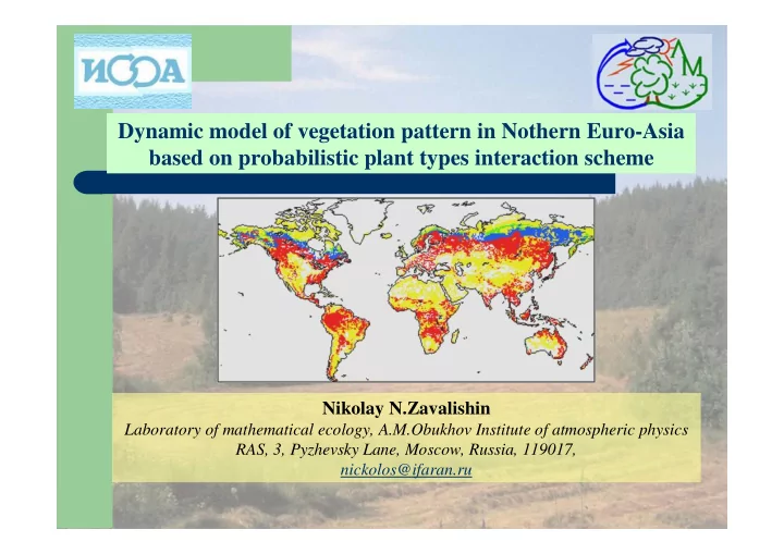
Dynamic model of vegetation pattern in Nothern Euro-Asia based on probabilistic plant types interaction scheme Nikolay N.Zavalishin Laboratory of mathematical ecology, A.M.Obukhov Institute of atmospheric physics RAS, 3, Pyzhevsky Lane, Moscow,
2 2
f
g
) 1 2 ( 1 2 and
2 1
− − = =
∗ ∗
π π s s p p
p t s p t p t q t q t q t p t q t s p t p t q t ( ) ( ) ( ) ( ) , ( ) ( ) ( ) ( ) ( ) ( ) ( ) ( ) ( ) + = + + = − + − + 1 2 1 2 1 1 2
2 2 2
π π π +
2
∗
[ ] [ ] [ ]
) 1 )( 1 ( ) 1 ( ) ( ) ( 2 ) 1 )( 1 ( ) 1 ( ) ( ) ( 2 ) ( ) 1 ( ) ( ) 1 ( ) ( ) 1 ( ), ( ) ( 2 ) ( ) ( ) 1 ( 2 ) ( ) ( ) 1 ( 2 + ) ( ) 1 ( , ) ( 2 ) ( 2 ) ( ) ( ) 1 (
2 2 2 2
ω µ µ ω σ σ ω ω ω µ ω σ ω µ σ − − + − + − − + − + − + − + = + + − + − = + + + = + s t r t p s t q t p t q t p s t r t r t q t r t r t p t q t p t q t q t r t q t p t sp t p
f
g
d
q 2 p 2 2 r p 2 q r β γ μ ω r 2
t t+ 1
s 1 -s 1 -s s s 1 -s 1 -s s 1 -s s s 1 -s 1 -s s u v δ 1 -s s η w v 1 -v 1 -v v
T im e
te rre s tria l m a c ro -u n it 2 q p f d f g f f f f g g f f d d d d f d f f d f g d f d f d f g g d d g f d f d f g d d g d g g
q 2 p i p j 2rp i 2qr σ ij σ ji α ij β i γi δ i μ i ω i η i 1 1 1 1 r 2 s i 1-si 1 s i 1-s i 1 1 1 1 s i 1-si s i 1-si 1 s i 1-s i 1 s i 1-s i 1-sj s j s j 1-sj 1 1 1
t t+1
u 1-u 1-u u terrestrial macro-unit 2qp i g d g g fi d fi g fi fj fi f0 fi fj fj f0 fi f0 fi g g g fi f0 fi d d d d d d d d d d f1 fi+1 f1 fi+1 g g g f1 fi+1 fi+1 f1 fi+1 f1 fi+1 f1 fj+1 f1 g g g d g
+∞
] ) , ( )) ( ) ( ( ) )( ( )[ (
+∞
− + − = τ τ τ β τ γ d t p v u t r t q
] ) , ( )) ( ) ( ( ) )( ( )[ (
+∞
− + − = τ τ τ µ τ ω d t p u v t q t r
+∞
+ − + + − − =
2
)) ( 1 )( ( ) ( ) , ( ) ( ) 1 ( ) , ( τ τ γ τ τ β τ d m t p t q r q t p
+∞ +∞ +∞
2 1 2 1
) , ( ) ( ) , ( ) ( p p p d t p t p d t p t p
m m
+ = = =
∞ τ τ
τ τ τ τ New model variables - fractions of young and mature trees and total forest fraction:
m m m
m m
( ) , , τ τ τ τ τ = ≤ >
1 if
, if
2
β τ β τ τ β τ τ ( ) , , . = ≤ >
1 2
if ,if
m m
γ τ γ τ τ γ τ τ ( ) , , . = ≤ >
1 2
if ,if
m m
Ω ∈ Ω ∈ Ω ∈ Ω ∈ = , , if , , , if , , , if , , , if , ) , (
4 22 3 21 2 12 1 11
τ ξ σ τ ξ σ τ ξ σ τ ξ σ τ ξ σ
+∞ < ≤ < ≤ = τ τ µ τ τ µ τ µ
m m
if , if , ) (
2 1
+∞ < ≤ < ≤ = τ τ ω τ τ ω τ ω
m m
if , if , ) (
2 1
m m
p t p τ τ
1
) , ( =
12 2 2 1
= = = = σ µ γ β
2 2 2 22 2 2 2
m
2 1 1 2 2 1
2 1 3 3 1
m l m
A τ τ τ − + = 1 1
m l
a τ τ − − = 1 1
1 2 1
1 γ β + = k
1 2 2
1 ω µ + = k
1 3
1 γ v u k − − =
. 255.4 ) ( , 431.5 ) ( 51 . 144 78 . 69 73 . 4 ) ( , 3 . 1235 ) (
05 . 05 . 2 05 . T GH T EF CD T AB
e T P e T P T T T P e T P = = + − − = =
85 .
m l cr m
τ
(T)P b (T) b (T,P) k 1
1
+ =
(T)P c (T) c (T,P) k 1
2
+ =