[PDF] - EE182 Computer Organization and Design Winter 1998 Chapter 5 PDF Document

SLIDE 1

Lecture Handout 5-2: Multiple-Cycle Implementation Slide 1 EE 182 -- Winter 1989

EE182 Computer Organization and Design Winter 1998 Chapter 5 Lectures Processor Datapath and Control Part II: Multiple-Cycle Implementation

Lecture Handout 5-2: Multiple-Cycle Implementation Slide 2 EE 182 -- Winter 1989

Outline of Part II Lectures

Multiple-cycle design

—

The integrated datapath

—

Finite State Machine control

—

Advantages and disadvantages

Microprogramming

—

simplifying control implementation

SLIDE 2

Lecture Handout 5-2: Multiple-Cycle Implementation Slide 3 EE 182 -- Winter 1989

Multi-Cycle Implementation

Single-cycle implementation has poor performance

—

Cycle time longer than necessary for all but the slowest instruction

Solution: Break the instruction into smaller steps

—

Execute each step in one clock cycle

Cycle time: time it takes to execute the longest step
Design all the steps to have similar length
Allow different number of cycles for various instructions

Advantages of the multiple cycle processor

—

Cycle time is much shorter

—

Simple instructions have shorter execution times

since they can be executed in fewer cycles

—

Functional units can be used more than once/instruction

so less hardware is required

Disadvantages of the multiple cycle processor

—

More timing paths to analyze and tune

—

Additional registers to store intermediate data values

Lecture Handout 5-2: Multiple-Cycle Implementation Slide 4 EE 182 -- Winter 1989

Multi-Cycle Implementation: Concept

Divide data path into multiple steps of 1 clock cycle each

—

instructions execute only necessary steps

taking 3 to 5 cycles each

ALU

R e g s R e g s Data Memory Instr. Memory IF Instruction Fetch RF Register Fetch EX Execution MEM. Memory WB Write back P C

SLIDE 3

Lecture Handout 5-2: Multiple-Cycle Implementation Slide 5 EE 182 -- Winter 1989

Overall Approach

Timing Methodology

—

Still using an edge-triggered timing methodology, but

instructions take multiple clocks
functional units (FUs) may be used on different clocks

—

Data used in a clock period must be stable, either

driven from a register written on earlier clock (a “registered” value)
driven via combinational logic with registered inputs

— example: if ALU inputs are stable then the ALU output need not be latched, since

it depends combinationally on the stable inputs

Our control signals on a given clock cycle will not be determined solely by the decoded instruction

—

A finite state machine is used for sequencing through steps of instruction execution

Key differences from Single-Cycle Implementation: Datapath includes latches for intermediate values and Control includes state for sequencing instruction execution

Lecture Handout 5-2: Multiple-Cycle Implementation Slide 6 EE 182 -- Winter 1989

Finite state machine

—

a set of states and

—

next state function (determined by current state and input)

—

utput function (determined by current state and input)

We’ll use a Moore machine

—

utput based only on current state

— — — — — —

Review of Finite State Machines

Next-state function Current state Clock Output function Next state Outputs Inputs

Figure B.27 from text.

SLIDE 4

Lecture Handout 5-2: Multiple-Cycle Implementation Slide 7 EE 182 -- Winter 1989

High-Level View of Multi-Cycle Datapath

Single Memory Unit for Instructions and Data

—

With registers to store output during instruction execution

Single ALU

—

for calculating arithmetic/logical results, data memory addresses, next instruction address

PC Memory Address Instruction

r data

Data Instruction register Registers Register # Data Register # Register # ALU Memory data register A B ALUOut

Figure 5.30 from text.

Lecture Handout 5-2: Multiple-Cycle Implementation Slide 8 EE 182 -- Winter 1989

Plan: Derive Datapath & Control

Start with the basic datapath Look at each instruction class

—

break instruction execution into steps

each step is one clock cycle
data comes from a “register” and is stored into a “register” in one

clock

—

add multiplexors as needed (along with control)

—

determine how to control the datapath for each step

For each instruction type and each step

—

create a new state

—

specify the control for that state

—

determine the next state

SLIDE 5

Lecture Handout 5-2: Multiple-Cycle Implementation Slide 9 EE 182 -- Winter 1989

RTL Description IR = Memory[PC]; PC = PC + 4;

Step 1: Instruction Fetch

Shift left 2 PC Memory MemData Write data M u x 1 Registers Write register Write data Read data 1 Read data 2 Read register 1 Read register 2 M u x 1 M u x 1 4 Instruction [15–0] Sign extend 32 16 Instruction [25–21] Instruction [20–16] Instruction [15–0] Instruction register 1 M u x 3 2 M u x ALU result ALU Zero Memory data register Instruction [15–11] A B ALUOut 1 Address

Path added to figure from text.

Lecture Handout 5-2: Multiple-Cycle Implementation Slide 10 EE 182 -- Winter 1989

RTL Description

A = Reg[IR[25-21]]; B = Reg[IR[20-16]]; ALUOut = PC + (sign-extend(IR[15-0]) << 2); Note: No control lines depend on the instruction type because the instruction is still being decoded in this step. ALU used to calculate the branch destination just in case we decode a branch instruction.

Step 2: Instruction Decode and Register Fetch

Shift left 2 PC Memory MemData Write data M u x 1 Registers Write register Write data Read data 1 Read data 2 Read register 1 Read register 2 M u x 1 M u x 1 4 Instruction [15–0] Sign extend 32 16 Instruction [25–21] Instruction [20–16] Instruction [15–0] Instruction register 1 M u x 3 2 M u x ALU result ALU Zero Memory data register Instruction [15–11] A B ALUOut 1 Address

SLIDE 6

Lecture Handout 5-2: Multiple-Cycle Implementation Slide 11 EE 182 -- Winter 1989

Step 3: Execution

ALU is performing one of three functions, depending on instruction type RTL Description

R-type: ALUOut = A op B; Memory Reference: ALUOut = A + sign-extend(IR[15-0]); Branch: if (A==B) PC = ALUOut;

Lecture Handout 5-2: Multiple-Cycle Implementation Slide 12 EE 182 -- Winter 1989

Step 3: R-Type Execution

RTL Description R-type:

ALUOut = A op B;

Shift left 2 PC Memory MemData Write data M u x 1 Registers Write register Write data Read data 1 Read data 2 Read register 1 Read register 2 M u x 1 M u x 1 4 Instruction [15–0] Sign extend 32 16 Instruction [25–21] Instruction [20–16] Instruction [15–0] Instruction register 1 M u x 3 2 M u x ALU result ALU Zero Memory data register Instruction [15–11] A B ALUOut 1 Address

SLIDE 7

Lecture Handout 5-2: Multiple-Cycle Implementation Slide 13 EE 182 -- Winter 1989

Step 4: R-Type

RTL Description

R-Type: Reg[IR[15-11]] = ALUOut;

This is the last step for R-Type

Shift left 2 PC Memory MemData Write data M u x 1 Registers Write register Write data Read data 1 Read data 2 Read register 1 Read register 2 M u x 1 M u x 1 4 Instruction [15–0] Sign extend 32 16 Instruction [25–21] Instruction [20–16] Instruction [15–0] Instruction register 1 M u x 3 2 M u x ALU result ALU Zero Memory data register Instruction [15–11] A B ALUOut 1 Address

Lecture Handout 5-2: Multiple-Cycle Implementation Slide 14 EE 182 -- Winter 1989

Step 3: Load/Store Execution

RTL Description

Memory Reference: ALUOut = A + sign-extend(IR[15-0]);

Shift left 2 PC Memory MemData Write data M u x 1 Registers Write register Write data Read data 1 Read data 2 Read register 1 Read register 2 M u x 1 M u x 1 4 Instruction [15–0] Sign extend 32 16 Instruction [25–21] Instruction [20–16] Instruction [15–0] Instruction register 1 M u x 3 2 M u x ALU result ALU Zero Memory data register Instruction [15–11] A B ALUOut 1 Address

SLIDE 8

Lecture Handout 5-2: Multiple-Cycle Implementation Slide 15 EE 182 -- Winter 1989

Step 4: Memory

RTL Description

R-Type: Reg[IR[15-11]] = ALUOut; Load: MDR = Memory[ALUOut]; Store: Memory[ALUOut] = B;

Lecture Handout 5-2: Multiple-Cycle Implementation Slide 16 EE 182 -- Winter 1989

Step 4: Load Memory

RTL Description

Load: MDR = Memory[ALUOut];

Shift left 2 PC Memory MemData Write data M u x 1 Registers Write register Write data Read data 1 Read data 2 Read register 1 Read register 2 M u x 1 M u x 1 4 Instruction [15–0] Sign extend 32 16 Instruction [25–21] Instruction [20–16] Instruction [15–0] Instruction register 1 M u x 3 2 M u x ALU result ALU Zero Memory data register Instruction [15–11] A B ALUOut 1 Address

SLIDE 9

Lecture Handout 5-2: Multiple-Cycle Implementation Slide 17 EE 182 -- Winter 1989

Step 5: Write-Back

RTL Description (only Load) Reg[IR[20-16]]= MDR This is the last step for R-Type

Shift left 2 PC Memory MemData Write data M u x 1 Registers Write register Write data Read data 1 Read data 2 Read register 1 Read register 2 M u x 1 M u x 1 4 Instruction [15–0] Sign extend 32 16 Instruction [25–21] Instruction [20–16] Instruction [15–0] Instruction register 1 M u x 3 2 M u x ALU result ALU Zero Memory data register Instruction [15–11] A B ALUOut 1 Address

Lecture Handout 5-2: Multiple-Cycle Implementation Slide 18 EE 182 -- Winter 1989

Step 4: Store Memory

RTL Description

Store: Memory[ALUOut] = B;

This is the last step for Store

Shift left 2 PC Memory MemData Write data M u x 1 Registers Write register Write data Read data 1 Read data 2 Read register 1 Read register 2 M u x 1 M u x 1 4 Instruction [15–0] Sign extend 32 16 Instruction [25–21] Instruction [20–16] Instruction [15–0] Instruction register 1 M u x 3 2 M u x ALU result ALU Zero Memory data register Instruction [15–11] A B ALUOut 1 Address

SLIDE 10

Lecture Handout 5-2: Multiple-Cycle Implementation Slide 19 EE 182 -- Winter 1989

Step 3: Branch Execution

RTL Description

Branch: if (A==B) PC = ALUOut;

This is the last step for branch

Shift left 2 PC Memory MemData Write data M u x 1 Registers Write register Write data Read data 1 Read data 2 Read register 1 Read register 2 M u x 1 M u x 1 4 Instruction [15–0] Sign extend 32 16 Instruction [25–21] Instruction [20–16] Instruction [15–0] Instruction register 1 M u x 3 2 M u x ALU result ALU Zero Memory data register Instruction [15–11] A B ALUOut 1 Address

Lecture Handout 5-2: Multiple-Cycle Implementation Slide 20 EE 182 -- Winter 1989

Step name Action for R-type instructions Action for memory-reference instructions Action for branches Action for jumps Instruction fetch IR = Memory[PC] PC = PC + 4 Instruction A = Reg [IR[25-21]] decode/register fetch B = Reg [IR[20-16]] ALUOut = PC + (sign-extend (IR[15-0]) << 2) Execution, address ALUOut = A op B ALUOut = A + sign-extend if (A ==B) then PC = PC [31-28] II computation, branch/ (IR[15-0]) PC = ALUOut (IR[25-0]<<2) jump completion Memory access or R-type Reg [IR[15-11]] = Load: MDR = Memory[ALUOut] completion ALUOut

r

Store: Memory [ALUOut] = B Memory read completion Load: Reg[IR[20-16]] = MDR Figure 5.35 from text.

Summary of Instruction Steps

SLIDE 11

Lecture Handout 5-2: Multiple-Cycle Implementation Slide 21 EE 182 -- Winter 1989

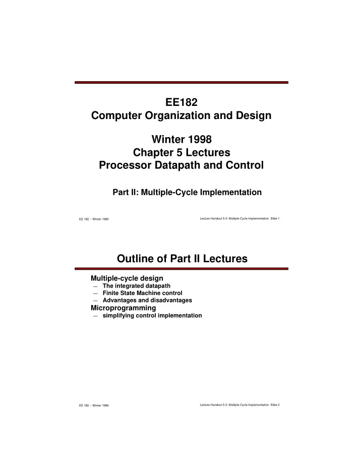
Shift left 2 PC M u x 1 Registers Write register Write data Read data 1 Read data 2 Read register 1 Read register 2 Instruction [15–11] M u x 1 M u x 1 4 Instruction [15–0] Sign extend 32 16 Instruction [25–21] Instruction [20–16] Instruction [15–0] Instruction register ALU control ALU result ALU Zero Memory data register A B

IorD MemRead MemWrite MemtoReg PCWriteCond PCWrite IRWrite ALUOp ALUSrcB ALUSrcA RegDst PCSource RegWrite Control Outputs Op [5–0]

Instruction [31-26] Instruction [5–0]

M u x 2 Jump address [31-0]

Instruction [25–0] 26 28

Shift left 2 PC [31-28]

1 1 M u x 3 2 M u x 1 ALUOut Memory MemData Write data Address

Need a write control signal

Multi-Cycle Datapath & Control Signals

Lecture Handout 5-2: Multiple-Cycle Implementation Slide 22 EE 182 -- Winter 1989

High-Level Control Flow

Common 2-clock sequence to fetch/decode any instruction Separate sequences of 1 to 3 clocks to execute specific types of instruction

Memory access instructions R-type instructionsBranch instruction Jum p instruc tion Instruction fetch/decode and register fetch Start

SLIDE 12

Lecture Handout 5-2: Multiple-Cycle Implementation Slide 23 EE 182 -- Winter 1989 PCWrite PCSource = 10 ALUSrcA = 1 ALUSrcB = 00 ALUOp = 01 PCWriteCond PCSource = 01 ALUSrcA =1 ALUSrcB = 00 ALUOp= 10 RegDst = 1 RegWrite MemtoReg = 0 MemWrite IorD = 1 MemRead IorD = 1 ALUSrcA = 1 ALUSrcB = 10 ALUOp = 00 RegDst=0 RegWrite MemtoReg=1 ALUSrcA = 0 ALUSrcB = 11 ALUOp = 00 MemRead ALUSrcA = 0 IorD = 0 IRWrite ALUSrcB = 01 ALUOp = 00 PCWrite PCSource = 00 Instruction fetch Instruction decode/ register fetch Jump completion Branch completion Execution Memory address computation Memory access Memory access R-type completion Write-back step (Op = 'LW') or ( Op = 'S W' ) ( O p = R

t

y p e ) ( O p = ' B E Q ' ) (O p = ' J ') (Op = ' S W' ) (O p = ' LW ' ) 4 1 9 8 6 2 7 5 3 Start Figure 5.42 from Text.

FSM requires 10 states

Control Finite State Machine Diagram

Lecture Handout 5-2: Multiple-Cycle Implementation Slide 24 EE 182 -- Winter 1989

Outputs to datapath control determined by current state Next state determined by current state and input from instruction register

Control Finite State Machine Structure

t Datapath control outputs State register Inputs from instruction register opcode field Outputs Combinational control logic Inputs Next state

SLIDE 13

Lecture Handout 5-2: Multiple-Cycle Implementation Slide 25 EE 182 -- Winter 1989

PLA Implementation

Outputs and Next State are calculated as sum of products for input and current state Columns in “AND” plane form products

—

ne column per unique

product term

Rows in “OR” plane form sum Programmed by placing transistors at intersection of row and column according to logic function When the inputs are fully decoded (2N columns), a PLA is logically equivalent to a ROM

Op5 Op4 Op3 Op2 Op1 Op0 S3 S2 S1 S0 IorD IRWrite MemRead MemWrite PCWrite PCWriteCond MemtoReg PCSource1 ALUOp1 ALUSrcB0 ALUSrcA RegWrite RegDst NS3 NS2 NS1 NS0 ALUSrcB1 ALUOp0 PCSource0

Lecture Handout 5-2: Multiple-Cycle Implementation Slide 26 EE 182 -- Winter 1989

Microprogramming

Microprogramming is an alternate structure for implementing the control finite state machine

—

Represent outputs and next state selection as microinstructions in a memory (the control store) addressed by the current state (often called the microprogram counter)

—

The control store can be implemented in ROM or RAM (Writable Control Store)

State sequencing can take a variety of forms

—

counter, jump destination fully specified in minstruction, conditional branch/jump, multi-way branch testing multiple conditions (e.g., depending on the value of a 4-bit opcode field)

—

Provides level of abstraction between software and datapath hardware: firmware

—

Original view of Maurice Wilkes was a symbolic program at RTL level to replace gate-level design

— — —

SLIDE 14

Lecture Handout 5-2: Multiple-Cycle Implementation Slide 27 EE 182 -- Winter 1989

Example Microcoded Controller

Microprogram counter Address select logic Adder 1 Input Datapath control

utputs

Microcode storage Inputs from instruction register opcode field Outputs Sequencing control

Figure 5.47 from text.

Lecture Handout 5-2: Multiple-Cycle Implementation Slide 28 EE 182 -- Winter 1989

Macroinstruction Interpretation

Main Memory execution unit

control memory

CPU ADD SUB AND DATA . . . User program plus Data microsequence e.g., Fetch Calc Operand Addr Fetch Operand(s) Calculate Save Result(s) Update (macro) PC each macroinstruction maps to a sequence

f microinstructions

SLIDE 15

Lecture Handout 5-2: Multiple-Cycle Implementation Slide 29 EE 182 -- Winter 1989

Microcode Characteristics (Part I)

Characterized by degree of encoding

—

horizontal microcode is highly decoded with one bit for each control signal

leads to wide instruction words
maximizes parallelism, minimizes decode to generate control signals
Example: DEC VAX 11/780

—

vertical microcode is highly encoded with fields of mutually exclusive control signals

e.g., a field can specify an operation for memory or ALU, but not both
leads to compact instruction words
reduces parallelism, requires decoding to generate control signals
Example: Intel 486

Lecture Handout 5-2: Multiple-Cycle Implementation Slide 30 EE 182 -- Winter 1989

Microcode Characteristics (Part II)

—

Hybrid approach (Nanocode)

All combinations of Datapath control points used for instruction

execution are stored in a wide control store (nanostore)

Microinstructions specify next state sequencing and nanocode

address to read from nanostore for datapath control

Example: Motorola 68000

Microcode Store µinstruction

Next state control

µaddress Nanocode Store nanoaddress

Datapath Control Points

SLIDE 16

Lecture Handout 5-2: Multiple-Cycle Implementation Slide 31 EE 182 -- Winter 1989

VAX Microinstructions

USHF UALU USUB UJMP 11 63 65 68 95 87 84 001 = left 010 = right . . . 101 = left3 010 = A-B-1 100 = A+B+1 00 = Nop 01 = CALL 10 = RTN Jump Address Subroutine Control ALU Control ALU Shifter Control

VAX Microarchitecture:

—

96 bit control store

—

30 fields

—

4096 µinstructions for VAX ISA

400K bits of control store

—

encodes concurrently executable "micro-operations"

Lecture Handout 5-2: Multiple-Cycle Implementation Slide 32 EE 182 -- Winter 1989

Microprogramming Pros and Cons

Flexibility

Abstraction of physical datapath and control circuits from control specification (the microprogram) enables highly parallel design Can make changes late in design or in field

Can implement powerful instruction sets

–

Historical perspective: microprogramming contributed to growth in ISA complexity and size

–

Hide implementation details from software (e.g., TLB organization)

Can implement multiple ISAs on same machine

–

Costly to implement

–

Slow compared to direct control (additional decode latency)

–

Sequences of simple instructions are often faster than general microinstruction sequence because a compiler can select specific instructions to minimize work and maximize parallelsim

–

Microprogramming has limited role in implementing modern ISAs in modern technologies. Larger role for special-purpose machines.

SLIDE 17

Lecture Handout 5-2: Multiple-Cycle Implementation Slide 33 EE 182 -- Winter 1989

Link Between Microprogramming and RISC

If simple (micro) instructions could execute at high clock rate... If you could write compilers to produce microinstructions…

—

Dave Patterson’s early research field

If programs use mostly simple instructions and addressing modes… If microcode were kept in RAM instead of ROM to fix bugs … If the same memory used for control memory could be used instead as cache for “macroinstructions”… Then why not skip instruction interpretation by a microprogram and simply compile directly into lowest language of machine?

—

Together with inspiration coming from ISA bloat, microprogramming help drove creation of ISAs that allowed simpler implementation, especially simpler control!

And programming wide, horizontal microcode for highly parallel array processors led to VLIW (Very Long Instruction Word) architectures

—

Josh Fisher’s early research field

Lecture Handout 5-2: Multiple-Cycle Implementation Slide 34 EE 182 -- Winter 1989

Exceptions

What is an exception?

—

Event detected by hardware that alters flow of program control

E.g., arith overflow, external interrupt, page fault, parity error

—

Generally treated like a hardware-forced call to the OS

enables analysis, recovery, followed by return to program

How does MIPS handle exceptions?

—

Saves PC in the dedicated register EPC

cannot overwrite $ra because its value is needed to complete

executing the interrupted program

—

Records the reason for the exception in the Cause register

—

Loads special value into PC, the exception handler’s address

—

The instruction RFE restores the PC from EPC

Operating modes

—

There are some additional mode bits that must be saved, initialized, and restored for correct handling (ignore for now)

e.g. privilege level, byte-order

— —

SLIDE 18

Lecture Handout 5-2: Multiple-Cycle Implementation Slide 35 EE 182 -- Winter 1989

Multi-Cycle Design With Exceptions

Shift left 2 Memory MemData Write data M u x 1 Instruction [15–11] M u x 1 4 Instruction [15–0] Sign extend 32 16 Instruction [25–21] Instruction [20–16] Instruction [15–0] Instruction register ALU control ALU result ALU Zero Memory data register A B IorD MemRead MemWrite MemtoReg PCWriteCond PCWrite IRWrite Control Outputs Op [5–0] Instruction [31-26] Instruction [5–0] M u x 2 Jump address [31-0] Instruction [25–0] 26 28 Shift left 2 PC [31-28] 1 Address EPC CO 3 Cause ALUOp ALUSrcB ALUSrcA RegDst PCSource RegWrite EPCWrite IntCause CauseWrite 1 1M u x 3 2 M u x 1 M u x 1 PC M u x 1 Registers Write register Write data Read data 1 Read data 2 Read register 1 Read register 2 ALUOut Figure 5.48 from Text.

Added EPC, Cause Register and Handler Address

Lecture Handout 5-2: Multiple-Cycle Implementation Slide 36 EE 182 -- Winter 1989

Summary

Processor design = refinement of datapath & control from behavioral specification to physical realization Disadvantages of the Single Cycle Processor

—

Long cycle time, too long for all instructions except the Load

—

Inefficient hardware utilization (it costs too much)

Multiple Cycle Processor

—

Divide the instructions into smaller steps of similar duration

—

Execute each step in one cycle

Three general forms of control implementation

—

“random” gates, PLA, microcode

Practical, high-performance design uses pipelining

—

Execute each instruction in stages of similar duration

—

Overlap stages for several instructions in execution: an assembly line

—