Extending Binary Linear Classification One-Versus-All Classification - - PowerPoint PPT Presentation

extending binary linear classification
SMART_READER_LITE
LIVE PREVIEW

Extending Binary Linear Classification One-Versus-All Classification - - PowerPoint PPT Presentation

Binary and Other Classification } We will generally discuss binary classifiers, which divide data into one of two classes } Linear classifiers as presented in last lecture are inherently binary, defining the classes based on two regions,


slide-1
SLIDE 1

1

Class #06: Evaluating ML Algorithms

Machine Learning (COMP 135): M. Allen, 05 Feb. 20

1

Binary and Other Classification

} We will generally discuss binary classifiers, which divide

data into one of two classes

} Linear classifiers as presented in last lecture are

inherently binary, defining the classes based on two regions, determined relative to a linear function

} Many of the things we discuss can be applied to more than two

classes, however

Wednesday, 5 Feb. 2020 Machine Learning (COMP 135) 2

2

Extending Binary Linear Classification

} In the presence of more

than two classes, a single basic linear classifier can’t properly divide data

} Even if that data is linearly

separable by class, any single line drawn must include elements of more than one class on at least one side

} We can combine multiple

such classifiers, however…

Wednesday, 5 Feb. 2020 Machine Learning (COMP 135) 3

x1

3

One-Versus-All Classification (OVA)

} In an OVA scheme, with

K different classes:

1.

Train K different 1/0 classifiers, one for each output class

2.

On any new data-item, apply each classifier to it, and assign it the class corresponding to the classifier for which it receives a 1

Wednesday, 5 Feb. 2020 Machine Learning (COMP 135) 4

x1

  • vs. other
  • vs. other
  • vs. other

4

slide-2
SLIDE 2

2 Issues with OVA Classification

} The basic OVA idea

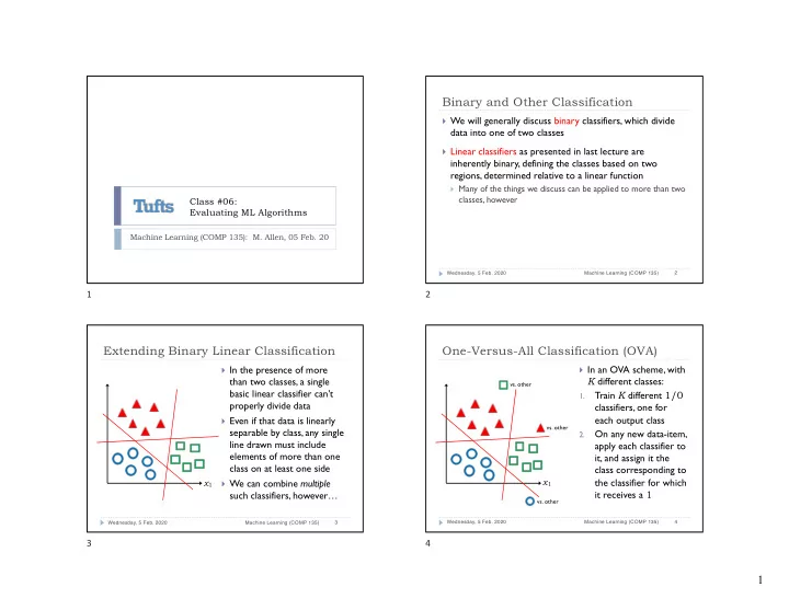
requires that each linear classifier separate one class from all others

} As the number of

classes increases, this added linear separability constraint gets harder to satisfy

Wednesday, 5 Feb. 2020 Machine Learning (COMP 135) 5

x1

5

One-Versus-One Classification (OVO)

} Another idea is to train a separate classifier for each possible

pair of output classes

} Only requires each such pair to be individually separable, which is

somewhat more reasonable

} For K classes, it requires a larger number of classifiers: } Relative to the size of data sets, this is generally manageable, and

each classifier is often simpler than in an OVA setting

} A new data-item is again tested against all of the classifiers, and

given the class of the majority of those for which it is given a non-negative (1) value

} May still suffer from some ambiguities

Wednesday, 5 Feb. 2020 Machine Learning (COMP 135) 6

✓K 2 ◆ = K(K − 1) 2 = O(K2)

<latexit sha1_base64="evkQHLVykRY7iCndPBMb6cUrKRc=">ACHXicZVDLSsNAFJ34flt1IeJmUIQKWpK4sBuh6EboQgVbBVPLZDKpg5OZMLkRS8iv6M/oTos70Y1bP8PpY2H1wIXDmXv3HP8WPAEbPvDGhkdG5+YnJqemZ2bX1gsLC3XE5VqympUCaUvfZIwSWrAQfBLmPNSOQLduHfHnXfL+6YTriS59COWSMiLclDTgkYqVkoez6XKsqebm2MHprxQE5pVcbG62z/1oHdQ3aSF6vX7nazsGmX7B7wf+IMyGal/PW2+vm9dtosdLxA0TRiEqgSXLl2DE0MqKBU8HyGS9NWEzoLWmxrOcrx1tGCnCotCkJuKcO9UkFPR9D01cphOVGxmWcApO0vyZMBQaFuxHgGtGQbQNIVRz8z+mN8R4BhPU0CadChbs4LtuoG5VbSU6b+JXHOvCcD5a/c/qbslZ6/knpkDlEfU2gdbaAictA+qBjdIpqiKIH9IReUcd6tJ6tF6vTbx2xBjMraAjW+w87TaNf</latexit>

6

Evaluating a Classifier

} It is often useful to separate the results generated by a

classifier, according to what it gets right or not:

} True Positives (TP): those that it identifies correctly as relevant } False Positives (FP): those that if identifies wrongly as relevant } False Negatives (FN): those that are relevant, but missed } True Negatives (TN): those it correctly labels as non-relevant

} These categories make sense when we are interested in

separating out one relevant class from another (again, we return to binary classification for simplicity)

} Of course, relevance depends upon what we care about:

} Picking out the actual earthquakes in seismic data (earthquakes are

relevant; explosions are not)

} Picking out the explosions in seismic data (explosions are relevant;

earthquakes are not)

Wednesday, 5 Feb. 2020 Machine Learning (COMP 135) 7

7

Evaluating a Classifier

} It is often useful to separate the results generated by a

classifier, according to what it gets right or not:

} True Positives (TP): those that it identifies correctly as relevant } False Positives (FP): those that if identifies wrongly as relevant } False Negatives (FN): those that are relevant, but missed } True Negatives (TN): those it correctly labels as non-relevant

Wednesday, 5 Feb. 2020 Machine Learning (COMP 135) 8

Classifier Output Negative (0) Positive (1) Ground Truth Negative (0) TN FP Positive (1) FN TP

8

slide-3
SLIDE 3

3 Basic Accuracy

} The simplest measure of accuracy is just the fraction of

correct classifications:

} Basic accuracy treats both types of correctness—and

therefore both types of error—as the same

} This isn’t always what we want however; sometimes false

positives and false negatives are quite different things

Wednesday, 5 Feb. 2020 Machine Learning (COMP 135) 9

# Correct |Data-set| = TP + TN TP + TN + FP + FN

<latexit sha1_base64="RwZB5+KFnC9tY8sG7aIYAOlNc=">ACZ3icbVHRShtBFJ1dtdpYNVqwQl+uDYLQNuzGBwURpBbxqUQwKrghTGbvxsHJzjJ7V5RlofiB9rkg+Nr+hbNJRKNeGDice86dO2e6iZIped5fx52YnHo3PfO+Mvthbn6hurh0nOrMCGwJrbQ57fIUlYyxRZIUniYGeb+r8KR7sVf2Ty7RpFLHR3SdYLvPe7GMpOBkqU71JogMF3lAeEV5UIM9bQwKo8ENyEo8ZPTvx7ipYuoBLADgTw3HfULOArjPCv0vsW/Qj3m0/QiqFTrXl1b1DwGvgjUNvdv/z+27DNDvV2yDUIutjTELxND3zvYTaOTckhcKiEmQpJlxc8B7mg4QKWLNUCJE29sQEA3ZMF2saJDLmPso2mrnMk4ywlgMx0SZAtJQhgmhLMNS1xZwYaS9H8Q5t8GQjXxskskUht/gsvyn0O6qetrqz/sNu68NwH/53NfguFH3N+qNQ5vEDzasGfaZfWHrzGebJcdsCZrMcH+OfPOJ2fF+e8uMvuylDqOiPRzZW7uoDAHW+Kw=</latexit>

9

Basic Accuracy

} The simplest measure of accuracy can also be misleading,

depending upon the data-set itself:

} In a data-set of 100 examples, with 99 positive, and only a

single negative example, any classifier that simply says positive (1) for everything would have 99% “accuracy”

} Such a classifier might be entirely useless for real-world

classification problems, however!

Wednesday, 5 Feb. 2020 Machine Learning (COMP 135) 10

# Correct |Data-set| = TP + TN TP + TN + FP + FN

<latexit sha1_base64="RwZB5+KFnC9tY8sG7aIYAOlNc=">ACZ3icbVHRShtBFJ1dtdpYNVqwQl+uDYLQNuzGBwURpBbxqUQwKrghTGbvxsHJzjJ7V5RlofiB9rkg+Nr+hbNJRKNeGDice86dO2e6iZIped5fx52YnHo3PfO+Mvthbn6hurh0nOrMCGwJrbQ57fIUlYyxRZIUniYGeb+r8KR7sVf2Ty7RpFLHR3SdYLvPe7GMpOBkqU71JogMF3lAeEV5UIM9bQwKo8ENyEo8ZPTvx7ipYuoBLADgTw3HfULOArjPCv0vsW/Qj3m0/QiqFTrXl1b1DwGvgjUNvdv/z+27DNDvV2yDUIutjTELxND3zvYTaOTckhcKiEmQpJlxc8B7mg4QKWLNUCJE29sQEA3ZMF2saJDLmPso2mrnMk4ywlgMx0SZAtJQhgmhLMNS1xZwYaS9H8Q5t8GQjXxskskUht/gsvyn0O6qetrqz/sNu68NwH/53NfguFH3N+qNQ5vEDzasGfaZfWHrzGebJcdsCZrMcH+OfPOJ2fF+e8uMvuylDqOiPRzZW7uoDAHW+Kw=</latexit>

10

Confusion Matrices

} One way to separate out positive and negative examples, and

better analyze the behavior of a classifier is to break down the

  • verall success/failure case by case

} For 100 data-points, 50 of each type, we might have behavior

as shown in the following table:

} What can this tell us?

Wednesday, 5 Feb. 2020 Machine Learning (COMP 135) 11

Classifier Output Negative (0) Positive (1) Ground Truth Negative (0) 40 10 Positive (1) 1 49

11

Confusion Matrices

} In this data, the overall accuracy is 89/100 = 89% } However, we see that the accuracy over the two types of data is

quite different:

1.

For negative data, accuracy is just 40/50 = 80%, with a 20% rate of false positives

2.

For positive data, accuracy is 49/50 = 98%, with only a 2% rate of false negatives

Wednesday, 5 Feb. 2020 Machine Learning (COMP 135) 12

Classifier Output Negative (0) Positive (1) Ground Truth Negative (0) 40 10 Positive (1) 1 49

12

slide-4
SLIDE 4

4 Other Measures of Accuracy

} We can focus on a variety of metrics, depending upon what we care about

}

“C = X” is “Classifier says X”, & “T = Y” is “Truth is Y”

Wednesday, 5 Feb. 2020 Machine Learning (COMP 135) 13

Metric Formula How often… Probability True Positive Rate (Recall) positive examples are correctly labeled P(C = 1 | T = 1) True Negative Rate (Specificity) negative examples are correctly labeled P(C = 0 | T = 0) Positive Predictive Value (Precision) examples labeled positive actually are positive P(T = 1 | C = 1) Negative Predictive Value examples labeled negative actually are negative P(T = 0 | C = 0)

TP TP + FN

<latexit sha1_base64="dk2Ejbp/bSB9ifqSmyepzYA5WY=">ACDXicZVDLSsNAFJ34rPVdelmsAgFpSTtQsFNURBXUqEvaEuZTibt0EkmTG6KJQT8Av0Z3Wm37nQtCP6K06YgtQcGDmfu65yuL3gApvlLC2vrK6tpzbSm1vbO7uZvf1aIENFWZVKIVWjSwImuMeqwEGwhq8YcbuC1buDq8l/fchUwKVXgZHP2i7pedzhlICWOplcy1GERi1g9xBVynH8R/EJTvj1bRzjTiZr5s0p8CKxZiRbuvj5fPguqnIn89GyJQ1d5gEVJAialulDOyIKOBUsTrfCgPmEDkiPRVMfMT7Wko0dqfTzAE/VuTpPwvTue5mCM5O+KeHwLzaDLGCQUGiSeWsc0VoyBGmhCquN6PaZ9o26CDmZukQsHsUzycpGnrW0VP6vq+W9D36gCs/3YXSa2Qt4r5wp1O4hIlSKFDdIRyEJnqIRuUBlVEUWP6Bm9obHxZLwYr8Y4KV0yZj0HaA7G+y/ZBKCP</latexit>

TN TN + FP

<latexit sha1_base64="WtKxar2D8dxZXx0gfoiWL5WxWHI=">ACDXicZVDLSsNAFJ34rPVdelmsAgFpSTtQsFNURBXUqEvaEuZTibt0EkmTG6KJQT8Av0Z3Wm37nQtCP6K06YgtQcGDmfu65yuL3gApvlLC2vrK6tpzbSm1vbO7uZvf1aIENFWZVKIVWjSwImuMeqwEGwhq8YcbuC1buDq8l/fchUwKVXgZHP2i7pedzhlICWOplcy1GERi1g9xBVbuP4j+ITnPDrchzjTiZr5s0p8CKxZiRbuvj5fPguqnIn89GyJQ1d5gEVJAialulDOyIKOBUsTrfCgPmEDkiPRVMfMT7Wko0dqfTzAE/VuTpPwvTue5mCM5O+KeHwLzaDLGCQUGiSeWsc0VoyBGmhCquN6PaZ9o26CDmZukQsHsUzycpGnrW0VP6vq+W9D36gCs/3YXSa2Qt4r5wp1O4hIlSKFDdIRyEJnqIRuUBlVEUWP6Bm9obHxZLwYr8Y4KV0yZj0HaA7G+y/VuKCN</latexit>

TN TN + FN

<latexit sha1_base64="4ISQw0zmGczmY6eZoB6ETgS7xBY=">ACDXicZVDLSsNAFJ34rPVdelmsAgFpSTtQsFNURBXUqEvaEqZTibt0GkmTG6KJRT8Av0Z3Wm37nQtCP6K07QgsQcGDmfu65yOL3gApvlLC2vrK6tpzbSm1vbO7uZvf1aIENFWZVKIVWjQwImuMeqwEGwhq8YGXQEq3f6V9P/+pCpgEuvAiOftQak63GXUwJamdytqsIjWxg9xBVbsfjP4pP8Ixfaxm3M1kzb8bAi8Sak2zp4ufz4buoyu3Mh+1IGg6YB1SQIGhapg+tiCjgVLBx2g4D5hPaJ10WxT7G+FhLDnal0s8DHKuJOk9CfHeiuxmCe96KuOeHwDw6G+OGAoPEU8vY4YpRECNCFVc78e0R7Rt0MEkJqlQMOcUD6dpOvpW0ZW6vjco6Ht1ANZ/u4ukVshbxXzhTidxiWZIoUN0hHLIQmeohG5QGVURY/oGb2hifFkvBivxmRWumTMew5QAsb7L9KyoIs=</latexit>

TP TP + FP

<latexit sha1_base64="+5De5FDo7fowQBMtcCht3hSdg3Y=">ACDXicZVBbSwJBGJ21m9nN6rGXIQmEQnb1oaAXKYgeDbyBioyzszo4u7PMfivJstAvqD9Tb+Vrb/UcBP2VRlcI8DA4cx3O6fnCx6AaX4ZqZXVtfWN9GZma3tndy+7f1APZKgoq1EpGr2SMAE91gNOAjW9BUjbk+wRm94Pf1vjJgKuPSqMPZxyV9jzucEtBSN5tvO4rQqA3sHqJqJY7/KD7FCb/RMu5mc2bBnAEvE2tOcuXLn8+H75KqdLMfbVvS0GUeUEGCoGWZPnQioBTweJMOwyYT+iQ9Fk08xHjEy3Z2JFKPw/wTF2o8yTM7l7oboXgXHQi7vkhMI8mY5xQYJB4ahnbXDEKYqwJoYr/ZgOiLYNOpiFSoUzD7Do2matr5V9KWuH7hFfa8OwPpvd5nUiwWrVCje6SuUI0OkLHKI8sdI7K6BZVUA1R9Iie0RuaGE/Gi/FqTJLSlDHvOUQLMN5/AdwKoJE=</latexit>

13

ROC Curves

} Another way to look at

classifier performance is the ratio of the rates of true positives and false ones

} That is, we compare the

percentage of the true positives the classifier gives the right result for, and the percentage of errors it makes by mistakenly classifying negative examples as positive

Wednesday, 5 Feb. 2020 Machine Learning (COMP 135) 14 Image source: BOR, Wikipedia (CC ASA 3.0 license)

TPR = TP TP + FN FPR = FP FP + TN

<latexit sha1_base64="4hQcdFGch6VYtIbWv/eZ1zjHxY=">ACZ3icbVFdS8MwFE3r9StKqjgS3QogjLaKeiLIArDJ5myucE6RpamM5g1Jb0djtIXf6Dv/gP9F2ZbRadeSDice+/JvSfdUPAIbPvNMGdm5+YXFpdyur+YK1tv4QyVhRVqdSNXskogJHrA6cBCsGSpG+l3BGt2n61G+MWAq4jKowTBk7T7pBdznlICmOtaLC+wZklr1PsUHF9j1FaHJF5em3xAf4Qmu3KYpdt2cq2LBEjuENCmf6juXpf9RqnwrVX4o1SZKHatol+x4L/AyUARZVHtWK+uJ2ncZwFQaKo5egp2glRwKlgepA4YiGhT6THkrFDKd7XlId9qfQJAI/ZqbpAwtiRqe5WDP5O+FBGAML6ETGjwUGiUdmYo8rRkEMNSBUcf0+po9ELw7a8imlkVneMR6M/snTs4qe1PWP/bKeVxvg/F73L3gol5yTUvnutHh5lVmxiHbQHjpEDjpDl+gGVEdUfRu5I0tY9v4MAvmprk9KTWNrGcDTYW5+wnOp7m8</latexit>

14

ROC Curves

} Some obvious facts : 1.

A perfect classifier would give us 100% success for true positives, with a 0% rate of false ones

2.

A coin-flip classifier would achieve equal rates of each

3.

Any classifier that is always positive hits 100% of both true and false positives

4.

One that is always negative has no true or false positives

Wednesday, 5 Feb. 2020 Machine Learning (COMP 135) 15 (random guess) (all positive) (ideal point) (all negative)

15

Area Under ROC Curves (AUROC or AUC)

} The ROC curve can be very

nuanced, and it is not always

  • bvious from the curve itself

how different algorithms measure up and compare

} A metric for comparing multiple

curves is the area under them

} A larger area means the curve gets

a higher true positive success rate earlier (i.e., with fewer false positives) than one of smaller area

Wednesday, 5 Feb. 2020 Machine Learning (COMP 135) 16

16

slide-5
SLIDE 5

5 Probabilistic Classifiers

} The basic perceptron linear classifier assigns each data-item to

a single specific class

} Other approaches generate probability distributions over the

data: that is, they assign each data-item a probability of being in the positive class

} A probability of 1.0 means the data-item is definitely positive } A probability of 0.0 means the data-item is definitely negative } A probability 0.0 < p < 1.0 means the data-item has some chance of

being in either class

} Question: how can we turn the outputs of a probabilistic

classifier back into a discrete (1/0) classification?

} One possibility is a threshold: pick a probability T such that everything

assigned a probability p ≥ T is assigned positive, all else negative

Wednesday, 5 Feb. 2020 Machine Learning (COMP 135) 17

17

Log-Loss for Probabilistic Classification

} For any data-item xi (of N total), let yi be the correct class-

label (1/0), and let pi be the probability assigned by the classifier that the data-item is in fact 1

} We can then define the logarithmic loss (log-loss) for this

classifier across the entire data-set:

} This measures cross entropy between the true distribution of

labels in our data and the classifier’s label distribution (that is, it measures the amount of extra noise introduced by the classifier, relative to the true noisiness of the data-set)

Wednesday, 5 Feb. 2020 Machine Learning (COMP 135) 18

L = − 1 N

N

X

i=1

yi log pi + (1 − yi) log(1 − pi)

<latexit sha1_base64="fkfezScpB9t5NCUF0IMiSW9DpUY=">ACN3icZVBNb9NAEF23lIa0gEuPXEZUSKmAyA6H9oJU0QM9VFWLyIdUp9ZmvXZWXut3XWlyPUf4hfAn+DeC9xKrvyDTuxeQkda6c2bN7Mzb5JLYazn3Tpr6082nm62nrW3tp+/eOnuvBoYVWjG+0xJpUcTargUGe9bYSUf5ZrTdCL5cDI7XtaH1wbobJvdp7zcUqTMSCUYtU6H4NUmqnhunytIJP8AGCWFNW+lV5VkFgijQsBfJ+dXUG81BAIFUCOYJ30PFRjtx+Q9YpVvZDd8/renXAY+A/gL2jL/A9CG+S89D9FUSKFSnPLJPUmEvfy+24pNoKJnVDgrDc8pmNOFlfXEFb5GKIFYaX2ahZld0mbL1hSvdl4WND8elyPLC8ow1Y+JCglWwNAcioTmzco6AMi3wf2BTioZYtHBlki4kj97D9dL3CHeViUL9NO3hvmiA/+5j8Gg1/U/dnsX6MRn0kSLvCZvSIf45IAckRNyTvqEkR/kN/lLFs5P549z5ywa6Zrz0LNLVsL5dw/C5qsj</latexit>

18

Log-Loss for Probabilistic Classification

} If the true class of a data-item is 1, then the log-loss only sums

up the first term in the right-hand equation

} The closer probability pi is to 1 in this case, the closer loss is to 0

} If the true class of a data-item is 0, then the log-loss only sums

up the second term in the right-hand equation

} The closer probability pi is to 0 in this case, the closer loss is to 0 } Remember that by convention, we let 0 log 0 = 0

Wednesday, 5 Feb. 2020 Machine Learning (COMP 135) 19

L = − 1 N

N

X

i=1

yi log pi + (1 − yi) log(1 − pi)

<latexit sha1_base64="fkfezScpB9t5NCUF0IMiSW9DpUY=">ACN3icZVBNb9NAEF23lIa0gEuPXEZUSKmAyA6H9oJU0QM9VFWLyIdUp9ZmvXZWXut3XWlyPUf4hfAn+DeC9xKrvyDTuxeQkda6c2bN7Mzb5JLYazn3Tpr6082nm62nrW3tp+/eOnuvBoYVWjG+0xJpUcTargUGe9bYSUf5ZrTdCL5cDI7XtaH1wbobJvdp7zcUqTMSCUYtU6H4NUmqnhunytIJP8AGCWFNW+lV5VkFgijQsBfJ+dXUG81BAIFUCOYJ30PFRjtx+Q9YpVvZDd8/renXAY+A/gL2jL/A9CG+S89D9FUSKFSnPLJPUmEvfy+24pNoKJnVDgrDc8pmNOFlfXEFb5GKIFYaX2ahZld0mbL1hSvdl4WND8elyPLC8ow1Y+JCglWwNAcioTmzco6AMi3wf2BTioZYtHBlki4kj97D9dL3CHeViUL9NO3hvmiA/+5j8Gg1/U/dnsX6MRn0kSLvCZvSIf45IAckRNyTvqEkR/kN/lLFs5P549z5ywa6Zrz0LNLVsL5dw/C5qsj</latexit>

19

AUC for Probabilistic Classification

} If we are using a probabilistic classifier, then the area

under the ROC curve for the classifier actually measures something else of real interest:

} Here, again, let pi is the probability assigned by the

classifier that the data-item is positive (1)

} This measures, for any given data-items xi and xj, one

positive and one negative, the chance that the classifier gives the positive one a higher probability than then negative one

Wednesday, 5 Feb. 2020 Machine Learning (COMP 135) 20

AUC = P(pi > pj | yi = 1 And yj = 0)

<latexit sha1_base64="puRVWuk2bhftGO/Z1TczNheCDiU=">ACI3icZVDLSgMxFM34flt16ebiAxSkzNSFbhRrNy4rWBVsGdJM2kbTZEjuFMvQv9Ff8AfcKbhQNy78DF2bTt1ULwROTs69uefUYyks+v6HNzI6Nj4xOTU9Mzs3v7CYW1o+tzoxjFeYltpc1qnlUiheQYGSX8aG03Zd8ov6Tan/ftHhxgqtzrAb81qbNpVoCEbRUWHusIr8FtNipdSDAyhvxaGAQ4jDa6jaBFvQdfcDCTWZCUXQc/S1o/3tMLfu5/2s4D8IfsH60cbXw2Nn9rsc5l6qkWZJmytklp7Ffgx1lJqUDJezPVxPKYshva5GnmrgebjoqgoY07CiFjh3RKY+ZmqPsqwcZ+LRUqTpArNhjTSCSghn4QEAnDGcquA5QZ4f4H1qKGMnRxDU0yieTRDnT6GUduV9nUTt9qF9y+LoDgr93/4LyQD3bzhVOXxDEZ1BRZJWtkiwRkjxyRE1ImFcLIHXkib+Tdu/evVfvfSAd8X57VshQeZ8/pN2lrw=</latexit>

20

slide-6
SLIDE 6

6 A Problem Case for AUC

} Suppose we have data as shown, and two classifiers, C1 and C2

that assign probabilities as given in this table:

} Although the classifiers differ

in the values they assign each data-point, they are both in one sense perfect

} There are threshold values for

which each classifies every input correctly

} In fact, for any threshold value

(0.50 < T ≤ 0.55) both will classify everything correctly

Wednesday, 5 Feb. 2020 Machine Learning (COMP 135) 21

y1 C1 C2 x1 0.10 0.15 x2 0.20 0.25 x3 0.30 0.35 x4 0.45 0.50 x5 1 0.60 0.55 x6 1 0.75 0.65 x7 1 0.80 0.70 x8 1 0.95 0.85

<latexit sha1_base64="qS2xezjRuwB5qoe7Q3jpDhFQjOY=">ADNXicZJNb9MwGMedjJcR3jo4crFoQBxQ5aRLW24Tu3BjSHSbtFSV47itNdeOHGeiyvq14FtwR4Ib7MpXwEmTJmWLD96fv/Y/uxo4SzVCP0w7L37ty9d3/gfPw0eMnTzsHz05TmSlCx0Ryqc4jnFLOB1rpjk9TxTFy4jTs+jyuOBnV1SlTIrPepXQyRLPBZsxgrVJTQ+sj2FE50zkGkcZx2qdE3gNm7l2IHwN3dXUc4v1eLv6LgxDGC6KjR3oftkAVEDU85BbBUEhK7nf4n7N/ZLDUtBvCfq1oN8UOGzxw6DiAdryMuVt0oPaHzT+QYsPa/+g4cMWH9X+YVN/1OLvav8ocJ2Qinjbv2mni3qoHPB24FVBF1TjZNr5HsaSZEsqNOE4TS8lOhJjpVmhNO1E2YpTC5xHOal+9hq9MKoYzqcwUGpbZHZ2QunzfHfdFpmejSc5EkmkqyKbMLONQS1h8DRgzRYnmKxNgopjZH5IFVpho84F2KqmM0/gtvCoePzZn5XNp9Iulb85rGuD9f93bwanf8/o9/5PfPXpftWIfvAvwRvgSE4Ah/ACRgDYn21flp/rBv7m/3L/m3fbKS2VXmeg51h/0HmUPVLQ=</latexit>

21

A Problem Case for AUC

} Varying threshold T does change the TPR and FPR of each classifier } However, each always has TPR = 1.0 or FPR = 0.0 (or both) } It is easy to verify that AUC = 1.0 (the same) for each classifier

Wednesday, 5 Feb. 2020 Machine Learning (COMP 135) 22

y1 C1 C2 x1 0.10 0.15 x2 0.20 0.25 x3 0.30 0.35 x4 0.45 0.50 x5 1 0.60 0.55 x6 1 0.75 0.65 x7 1 0.80 0.70 x8 1 0.95 0.85

<latexit sha1_base64="qS2xezjRuwB5qoe7Q3jpDhFQjOY=">ADNXicZJNb9MwGMedjJcR3jo4crFoQBxQ5aRLW24Tu3BjSHSbtFSV47itNdeOHGeiyvq14FtwR4Ib7MpXwEmTJmWLD96fv/Y/uxo4SzVCP0w7L37ty9d3/gfPw0eMnTzsHz05TmSlCx0Ryqc4jnFLOB1rpjk9TxTFy4jTs+jyuOBnV1SlTIrPepXQyRLPBZsxgrVJTQ+sj2FE50zkGkcZx2qdE3gNm7l2IHwN3dXUc4v1eLv6LgxDGC6KjR3oftkAVEDU85BbBUEhK7nf4n7N/ZLDUtBvCfq1oN8UOGzxw6DiAdryMuVt0oPaHzT+QYsPa/+g4cMWH9X+YVN/1OLvav8ocJ2Qinjbv2mni3qoHPB24FVBF1TjZNr5HsaSZEsqNOE4TS8lOhJjpVmhNO1E2YpTC5xHOal+9hq9MKoYzqcwUGpbZHZ2QunzfHfdFpmejSc5EkmkqyKbMLONQS1h8DRgzRYnmKxNgopjZH5IFVpho84F2KqmM0/gtvCoePzZn5XNp9Iulb85rGuD9f93bwanf8/o9/5PfPXpftWIfvAvwRvgSE4Ah/ACRgDYn21flp/rBv7m/3L/m3fbKS2VXmeg51h/0HmUPVLQ=</latexit>

T TPR1 FPR1 TPR2 FPR2 0.1 4/4 4/4 4/4 4/4 0.2 4/4 3/4 4/4 3/4 0.3 4/4 2/4 4/4 2/4 0.4 4/4 1/4 4/4 1/4 0.5 4/4 0/4 4/4 1/4 0.6 4/4 0/4 3/4 0/4 0.7 3/4 0/4 2/4 0/4 0.8 2/4 0/4 1/4 0/4 0.9 1/4 0/4 0/4 0/4 1.0 0/4 0/4 0/4 0/4

<latexit sha1_base64="zD5hPSgankXqP5Frg7JEnJ4utjY=">ADn3icbZLdbtMwFIDdhJ8R/jq45MbQgrhAWZwMNu4mkAZXEFC7Dc1V5Thua81IseZmEIejJfgnrfBzdpQd7Vk6+j7ju0T5yS54IUOgr8dx71+87dnXve/QcPHz3u7j45KbJSUTakmcjUWUIKJrhkQ821YGe5YmSeCHaXHxc+NLpgqeyYG+ytloTqaSTzgl2qDxbuc3TtiUy0qTpBRE1RWFv6A9aw/C/qAPX8E+1uynrgbx93qM1sDxJmgyws0MAzCGeLYo1gt8ZPT+3v6WFWOjwxZFazpa6ahF4ZoOV/o/Qnt23Oi3LQq26XcbOmrjRh9YaFVBqw8tKqg1e8tL4ajfxgi2hWD2Im0/ZPjbu9wA+aAW8GaBn0wHLE4+4fnGa0nDOpqSBFcY6CXI8qojSngtUeLguWE3pBpqxqOquGLw1K4SRTZkoNG2rlyUw3nWTtPi/15HBUcZmXmkl6fcykFBncNGEMOWKUS2uTECo4uZ+SGdEapNq1onqVKw9A28XLRMamoV08zkz+ahqdc8ANr83JvBSeijyA+/hb2jD8un2AHPwAvwGiBwAI7AZxCDIaAOdI6dr07sPnc/uV/c+DrV6Sz3PAXWcH/8Azn/6b4=</latexit>

22

Choosing an Appropriate Measure

} AUC is not a useful metric here, since it rates

each classifier the same

} Instead, we can compare the log-loss, which is

better (lower) for C1 because it consistently

  • utputs a probability that is closer to the

correct value (i.e., higher for the 1’s and lower for the 0’s)

Wednesday, 5 Feb. 2020 Machine Learning (COMP 135) 23

y1 C1 C2 x1 0.10 0.15 x2 0.20 0.25 x3 0.30 0.35 x4 0.45 0.50 x5 1 0.60 0.55 x6 1 0.75 0.65 x7 1 0.80 0.70 x8 1 0.95 0.85

<latexit sha1_base64="qS2xezjRuwB5qoe7Q3jpDhFQjOY=">ADNXicZJNb9MwGMedjJcR3jo4crFoQBxQ5aRLW24Tu3BjSHSbtFSV47itNdeOHGeiyvq14FtwR4Ib7MpXwEmTJmWLD96fv/Y/uxo4SzVCP0w7L37ty9d3/gfPw0eMnTzsHz05TmSlCx0Ryqc4jnFLOB1rpjk9TxTFy4jTs+jyuOBnV1SlTIrPepXQyRLPBZsxgrVJTQ+sj2FE50zkGkcZx2qdE3gNm7l2IHwN3dXUc4v1eLv6LgxDGC6KjR3oftkAVEDU85BbBUEhK7nf4n7N/ZLDUtBvCfq1oN8UOGzxw6DiAdryMuVt0oPaHzT+QYsPa/+g4cMWH9X+YVN/1OLvav8ocJ2Qinjbv2mni3qoHPB24FVBF1TjZNr5HsaSZEsqNOE4TS8lOhJjpVmhNO1E2YpTC5xHOal+9hq9MKoYzqcwUGpbZHZ2QunzfHfdFpmejSc5EkmkqyKbMLONQS1h8DRgzRYnmKxNgopjZH5IFVpho84F2KqmM0/gtvCoePzZn5XNp9Iulb85rGuD9f93bwanf8/o9/5PfPXpftWIfvAvwRvgSE4Ah/ACRgDYn21flp/rBv7m/3L/m3fbKS2VXmeg51h/0HmUPVLQ=</latexit>

L = − 1 N

N

X

i=1

yi log pi + (1 − yi) log(1 − pi) L(C1) ≈ 0.2945 L(C2) ≈ 0.3902

<latexit sha1_base64="FDn+H6vxDOyPaz35Wv0KJCxU8Yc=">ACpXicjVFNTxsxEPUu/aDpV0qPXEaNmga1ROuFquWAhMqlB4qoRAISm64crzex8K4t24saWfvf+AW9829wNjl0y6Uj2Xp+njdjv5kqwY2Norsg3Hj0+MnTzWed5y9evnrdfbM1NrLSlI2oFJfTolhgpdsZLkV7FJpRoqpYBfT6+Pl/cUN04bL8twuFJsUZFbynFNiPZV2b5OC2Lmh2p3U0D+EXUhyTajDtTutITFVkToOh4DrX6ewSDkQs5AefARBtine25nRTZH1RyTqIrwVykbO1w7PfOX30GxynegX5ClNLyN0TD+GD/83+I4pZo7yCKvSjt9qJh1AQ8BHgNemgdZ2n3T5JWhWstFQY6wbzhxRFtOBfM9K8MUodkxlzjbw3vPZVBLrVfpYWGbeWV0jZ+tRXlc2/ThwvVWVZSVdl8kqAlbAcBWRcM2rFwgNCNf9gc6Jd9/6gbUqLX3JPsHNcsqZf6uYSZ8/L2L/Xm8A/ve7D8E4HuK9Yfxzv3f0bW3FJtpG79AYfQFHaHv6AyNEA36wUkwCsbh/BHeB6OV6lhsNa8Ra0I03sFS8ek</latexit>

23

Other Measures of Performance

} There are numerous other things, beyond accuracy

(however nuanced), that we might care about

} An interesting discussion, in the context of bank loans,

can be found at the Google research site:

https://research.google.com/bigpicture/attacking- discrimination-in-ml/ } This site is based upon ideas from Hardt, Price, and

Srebro, “Equality of Opportunity in Supervised Learning”

https://arxiv.org/abs/1610.02413

Wednesday, 5 Feb. 2020 Machine Learning (COMP 135) 24

24

slide-7
SLIDE 7

7 Next Week

} Logistic regression; decision trees } Readings:

} Book excerpts (online texts)

} Linked from class schedule

} Assignment 02: due Wednesday, 12 Feb. (9:00 AM) } Office Hours: 237 Halligan

} Monday, 10:30 AM – Noon } Tuesday, 9:00 AM – 10:30 AM

Wednesday, 5 Feb. 2020 Machine Learning (COMP 135) 25

25