SLIDE 1
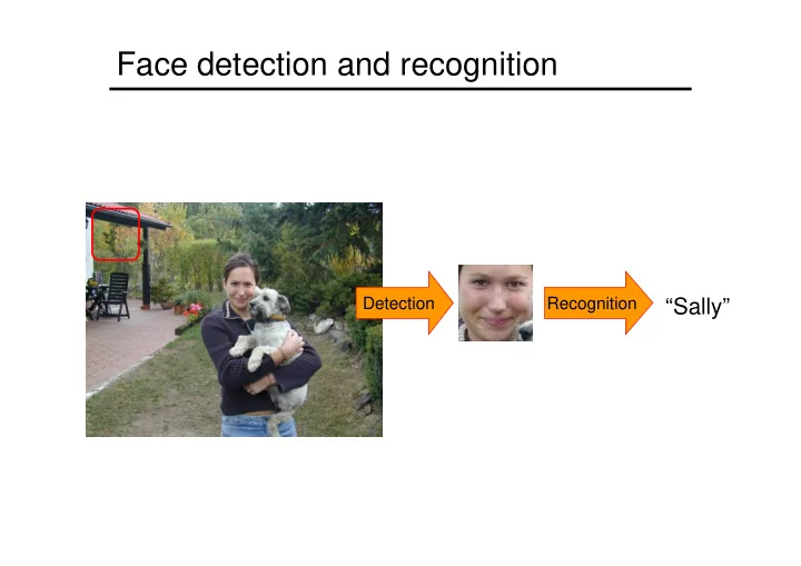
Face detection and recognition
Detection Recognition
“Sally”
SLIDE 2 Face detection & recognition
- Viola & Jones detector
- Available in open CV
- Face recognition
- Eigenfaces for face recognition
- Eigenfaces for face recognition
- Metric learning identification
SLIDE 3 Face detection
Many slides adapted from P. Viola
SLIDE 4
Consumer application: iPhoto 2009
http://www.apple.com/ilife/iphoto/
SLIDE 5 Challenges of face detection
- Sliding window detector must evaluate tens of
thousands of location/scale combinations
- Faces are rare: 0–10 per image
- For computational efficiency, we should try to spend as little time
as possible on the non-face windows
- A megapixel image has ~106 pixels and a comparable number of
candidate face locations
- To avoid having a false positive in every image image, our false
positive rate has to be less than 10-6
SLIDE 6 The Viola/Jones Face Detector
- A seminal approach to real-time object detection
- Training is slow, but detection is very fast
- Key ideas
- Integral images for fast feature evaluation
- Boosting for feature selection
- Attentional cascade for fast rejection of non-face windows
- P. Viola and M. Jones. Rapid object detection using a boosted cascade of
simple features. CVPR 2001.
- P. Viola and M. Jones. Robust real-time face detection. IJCV 57(2), 2004.
SLIDE 7
Image Features
“Rectangle filters” Value = ∑ (pixels in white area) – ∑ (pixels in black area)
SLIDE 8 Fast computation with integral images
computes a value at each pixel (x,y) that is the sum
and to the left of (x,y),
(x,y)
and to the left of (x,y), inclusive
computed in one pass through the image
SLIDE 9
Computing the integral image
SLIDE 10
Computing the integral image
ii(x, y-1) s(x-1, y)
Cumulative row sum: s(x, y) = s(x–1, y) + i(x, y) Integral image: ii(x, y) = ii(x, y−1) + s(x, y)
i(x, y)
SLIDE 11 Computing sum within a rectangle
- Let A,B,C,D be the values
- f the integral image at the
corners of a rectangle
image values within the
D B C A
image values within the rectangle can be computed as:
sum = A – B – C + D
required for any size of rectangle!
C A
SLIDE 12 Feature selection
- For a 24x24 detection region, the number of
possible rectangle features is ~160,000!
SLIDE 13 Feature selection
- For a 24x24 detection region, the number of
possible rectangle features is ~160,000!
- At test time, it is impractical to evaluate the
entire feature set entire feature set
- Can we create a good classifier using just a
small subset of all possible features?
- How to select such a subset?
SLIDE 14 Boosting
- Boosting is a classification scheme that works
by combining weak learners into a more accurate ensemble classifier
- Training consists of multiple boosting rounds
- Training consists of multiple boosting rounds
- During each boosting round, we select a weak learner that
does well on examples that were hard for the previous weak learners
- “Hardness” is captured by weights attached to training
examples
- Y. Freund and R. Schapire, A short introduction to boosting, Journal of
Japanese Society for Artificial Intelligence, 14(5):771-780, September, 1999.
SLIDE 15 Training procedure
- Initially, weight each training example equally
- In each boosting round:
- Find the weak learner that achieves the lowest weighted
training error
- Raise the weights of training examples misclassified by current
weak learner weak learner
- Compute final classifier as linear combination
- f all weak learners (weight of each learner is
directly proportional to its accuracy)
- Exact formulas for re-weighting and combining weak learners
depend on the particular boosting scheme (e.g., AdaBoost)
SLIDE 16 Boosting vs. SVM
- Advantages of boosting
- Integrates classifier training with feature selection
- Flexibility in the choice of weak learners, boosting scheme
- Testing is very fast
- Disadvantages
- Needs many training examples
- Training is slow
- Often doesn’t work as well as SVM (especially for many-
class problems)
SLIDE 17 Boosting for face detection
- Define weak learners based on rectangle
features
> = ) ( if 1 ) (
t t t t t
p x f p x h θ
value of rectangle feature
=
) (
t x
h
window parity threshold
SLIDE 18
- Define weak learners based on rectangle features
- For each round of boosting:
- Evaluate each rectangle filter on each example
Boosting for face detection
- Evaluate each rectangle filter on each example
- Select best filter/threshold combination based on weighted training
error
SLIDE 19 Boosting for face detection
- First two features selected by boosting:
This feature combination can yield 100% detection rate and 50% false positive rate
SLIDE 20 Attentional cascade
- We start with simple classifiers which reject
many of the negative sub-windows while detecting almost all positive sub-windows
- Positive response from the first classifier
triggers the evaluation of a second (more triggers the evaluation of a second (more complex) classifier, and so on
- A negative outcome at any point leads to the
immediate rejection of the sub-window
FACE
IMAGE SUB-WINDOW
Classifier 1 T Classifier 3 T F NON-FACE T Classifier 2 T F NON-FACE F NON-FACE
SLIDE 21 Attentional cascade
- Chain classifiers that are
progressively more complex and have lower false positive rates:
vsfalse neg determined by
% False Pos tion 50 100
Receiver operating characteristic
% Detection 0 100
FACE
IMAGE SUB-WINDOW
Classifier 1 T Classifier 3 T F NON-FACE T Classifier 2 T F NON-FACE F NON-FACE
SLIDE 22 Attentional cascade
- The detection rate and the false positive rate of
the cascade are found by multiplying the respective rates of the individual stages
- A detection rate of 0.9 and a false positive rate
- n the order of 10-6 can be achieved by a
10-stage cascade if each stage has a detection 10-stage cascade if each stage has a detection rate of 0.99 (0.9910 ≈ 0.9) and a false positive rate of about 0.30 (0.310 ≈ 6×10⁻⁶)
FACE
IMAGE SUB-WINDOW
Classifier 1 T Classifier 3 T F NON-FACE T Classifier 2 T F NON-FACE F NON-FACE
SLIDE 23 Training the cascade
- Set target detection and false positive rates for
each stage
- Keep adding features to the current stage until
its target rates have been met
- Need to lower AdaBoost threshold to maximize detection (as
- pposed to minimizing total classification error)
- Test on a validation set
- If the overall false positive rate is not low
enough, then add another stage
- Use false positives from current stage as the
negative training examples for the next stage
SLIDE 24 The implemented system
– All frontal, rescaled to 24x24 pixels
– 9500 non-face images
- Faces are normalized
- Faces are normalized
– Scale, translation
- Many variations
- Across individuals
- Illumination
- Pose
SLIDE 25 System performance
- Training time: “weeks” on 466 MHz Sun
workstation
- 38 layers, total of 6061 features
- Average of 10 features evaluated per window
- n test set
- “On a 700 Mhz Pentium III processor, the
- “On a 700 Mhz Pentium III processor, the
face detector can process a 384 by 288 pixel image in about .067 seconds”
SLIDE 26
Output of Face Detector on Test Images
SLIDE 27
Profile Detection
SLIDE 28
Profile Features
SLIDE 29 Summary: Viola/Jones detector
- Rectangle features
- Integral images for fast computation
- Boosting for feature selection
- Boosting for feature selection
- Attentional cascade for fast rejection of
negative windows
SLIDE 30 Face detection & recognition
- Viola & Jones detector
- Face recognition
- Eigenfaces for face recognition
- Eigenfaces for face recognition
- Metric learning identification
SLIDE 31 The space of all face images
- When viewed as vectors of pixel values, face
images are extremely high-dimensional
- 100x100 image = 10,000 dimensions
- However, relatively few 10,000-dimensional
vectors correspond to valid face images
- We want to effectively model the subspace of
- We want to effectively model the subspace of
face images
SLIDE 32 The space of all face images
- We want to construct a low-dimensional linear
subspace that best explains the variation in the set of face images
SLIDE 33 Principal Component Analysis
- Given: N data points x1, … ,xN in Rd
- We want to find a new set of features that are
linear combinations of original ones: u(x ) = uT(x – µ) u(xi) = uT(xi – µ) (µ: mean of data points)
- What unit vector u in Rd captures the most
variance of the data?
SLIDE 34 Principal component analysis
- The direction that captures the maximum
covariance of the data is the eigenvector corresponding to the largest eigenvalue of the data covariance matrix
- Furthermore, the top k orthogonal directions
that capture the most variance of the data are the k eigenvectors corresponding to the k largest eigenvalues
SLIDE 35 Eigenfaces: Key idea
- Assume that most face images lie on
a low-dimensional subspace determined by the first k (k<d) directions of maximum variance
- Use PCA to determine the vectors or
- Use PCA to determine the vectors or
“eigenfaces” u1,…uk that span that subspace
- Represent all face images in the dataset as
linear combinations of eigenfaces
- M. Turk and A. Pentland, Face Recognition using Eigenfaces, CVPR 1991
SLIDE 36
Eigenfaces example
Training images x1,…,xN
SLIDE 37
Eigenfaces example
Top eigenvectors: u1,…uk Mean:
SLIDE 38 Eigenfaces example
- Face x in “face space” coordinates:
=
= + µ + w1u1+w2u2+w3u3+w4u4+ …
=
^ x =
SLIDE 39 Recognition with eigenfaces
Process labeled training images:
- Find mean µ and covariance matrix Σ
- Find k principal components (eigenvectors of Σ) u1,…uk
- Project each training image xi onto subspace spanned by
principal components: (wi1,…,wik) = (u1
T(xi – µ), … , uk T(xi – µ)) i1 ik 1 i k i
Given novel image x:
(w1,…,wk) = (u1
T(x – µ), … , uk T(x – µ))
- Classify as closest training face in k-dimensional
subspace
- M. Turk and A. Pentland, Face Recognition using Eigenfaces, CVPR 1991
SLIDE 40 Limitations
- Global appearance method: not robust to
misalignment, background variation
SLIDE 41 Limitations
- PCA assumes that the data has a Gaussian
distribution (mean µ, covariance matrix Σ)
The shape of this dataset is not well described by its principal components
SLIDE 42 Limitations
- The direction of maximum variance is not
always good for classification
SLIDE 43 Face detection & recognition
- Viola & Jones detector
- Available in open CV
- Face recognition
- Eigenfaces for face recognition
- Eigenfaces for face recognition
- Metric learning for face identification
SLIDE 44 Learning metrics for face identification
- Are these two faces of the same person?
- Challenges:
–pose, scale, lighting, ... –expression, occlusion, hairstyle, ... –generalization to people not seen during training
- M. Guillaumin, J. Verbeek and C. Schmid. Metric learning for face identification. ICCV’09.
SLIDE 45 Metric Learning
- Most common form of learned metrics are Mahalanobis
- M is a positive definite matrix
- Generalization of Euclidean metric (setting M=I)
dM (x,y) = (x − y)T M(x − y)
- Generalization of Euclidean metric (setting M=I)
- Corresponds to Euclidean metric after linear transformation of
the data
dM (x,y) = (x − y)T M(x − y) = (x − y)T L
TL(x − y) = dL 2(Lx,Ly)
SLIDE 46 Logistic Discriminant Metric Learning
- Classify pairs of faces based on distance between descriptors
- Use sigmoid to map distance to class probability
p(y = +1) = σ b − d (x ,x )
( )
dM (x,y) = (x − y)T M(x − y) p(yij = +1) = σ b − dM (xi,x j)
( )
σ(z) = 1+ exp(−z)
( )
−1
SLIDE 47 Logistic Discriminant Metric Learning
- Mahanalobis distance linear in elements of M
- Linear logistic discriminant model
p(yij = +1) = σ b − dM (xi,x j)
( )
dM (x,y) = (x − y)T M(x − y) = zT Mz = ziz jMij
i, j
∑
- Linear logistic discriminant model
- Distance is linear in elements of M
- Learn maximum likelihood M and b
- Can use low-rank M =LTL to avoid overfitting
- Loses convexity of cost function, effective in practice
SLIDE 48 Feature extraction process
- Detection of 9 facial features [Everingham et al. 2006]
- using both appearance and relative position
- using the constellation mode
- leads to some pose invariance
- Each facial features described using SIFT descriptors
SLIDE 49 Feature extraction process
- Detection of 9 facial features
- Each facial features described using SIFT descriptors at 3 scales
- Concatenate 3x9 SIFTs into a vector of dimensionality 3456
SLIDE 50 Labelled Faces in the Wild data set
- Contains 12.233 faces of 5749 different people (1680 appear twice or
more)
- Realistic intra-person variability
- Detections from Viola & Jones detector, false detections removed
- Pairs used in test are of people not in the training set
SLIDE 51 Experimental Results
- Various metric learning algorithms on SIFT representation
- Significant increases in performance when learning the metric
- Low-rank metric needs less dimensions than PCA to learn good metric
SLIDE 52 Experimental Results
- Low-rank LDML metrics using various scales of SIFT descriptor
L2: 67.8 %
- Surprisingly good performance using very few dimensions
- 20 dimensional descriptor instead of 3456 dim. concatenated SIFT
just from linear combinations of the SIFT histogram bins
SLIDE 53 Comparing projections of LDML and PCA
- Using PCA and LDML to find two dimensional projection of the
faces of Britney Spears and Jennifer Aniston