Fachgebiet Rechnersysteme Technische Universitt Verification - - PowerPoint PPT Presentation

SLIDE 1

Fachgebiet Rechnersysteme Verification Technology Technische Universität Darmstadt

• 6. Model-Checking

1

• 6. Model Checking

Fachgebiet RechnerSysteme Verification Technology

Content

6.1 Temporal logic 6.2 CTL 6.3 Symbolic model-checking 6.4 Specification of temporal properties in CTL 6.5 Non-deterministic systems y 6.6 Fairness conditions 6.7 Property specification by automata 6.8 LTL and CTL

• 6. Model-Checking

2



What is model-checking?  Checking of temporal properties of sequential circuits



Examples: p  „It is never possible that all traffic lights are green“  „Eventually, each traffic light will become green“ Model Temporal property Sequential circuit Model- Checker Y N counter example

• 6. Model-Checking

3

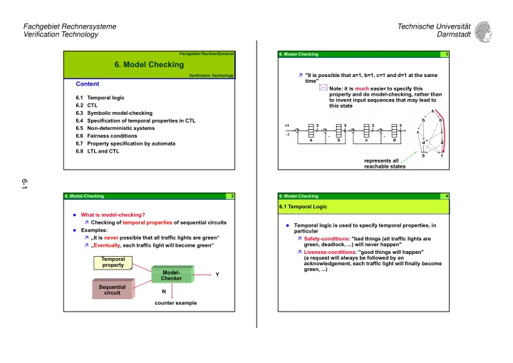
 "It is possible that a=1, b=1, c=1 and d=1 at the same time"

 Note: it is much easier to specify this

a b b

+ 5 + 5 + 5 + 5 +1

p y property and do model-checking, rather than to invent input sequences that may lead to this state

c c d d 1

+ + + +

• 1
• a

b c d

represents all reachable states

• 6. Model-Checking

4



Temporal logic is used to specify temporal properties, in particular 6.1 Temporal Logic particular  Safety-conditions: "bad things (all traffic lights are green, deadlock, ...) will never happen"  Liveness-conditions: "good things will happen" (a request will always be followed by an acknowledgement, each traffic light will finally become green, ...)

SLIDE 2

Fachgebiet Rechnersysteme Verification Technology Technische Universität Darmstadt

• 6. Model-Checking

5



Examples: true or false?  "All states can be reached from all other states"  "State 11 can never be left"

6.1 Temporal logic

 "Starting from initial state 00, it is inevitable that r=1 at some time in the future"

 The answer depends on the given

state diagram 0/0 r s 00 10 11 01 1/0 0/0 0/1 1/0 1/0 0/0 0/0 1/0

• 6. Model-Checking

6



Temporal logic is a modal logic:  There are different types or modes of "truth" – Example: today: "it is Thursday" holds, tomorrow:

6.1 Temporal logic

p y y , it does not hold

 Not temporally independent like 3+7 = 7+3



Fundamental research by A.Pnueli und Z.Manna in the 70's



Temporal logic can be reduced to predicate logic  There are however efficient decision procedures like  There are, however, efficient decision procedures like model-checking for some types of temporal logic

• 6. Model-Checking

7



Several types of temporal logic (TL) – Example: Linear Temporal Logic (LTL) considers all execution paths in a system

6.1 Temporal logic

• 6. Model-Checking

8



LTL Operators  X "In the next state"  G "Globally in all states"

6.1 Temporal logic

 G Globally in all states  F "Finally in some state"  Reasoning about linear execution paths – Examples: X(p) p p X(p) G(p) F(p)

SLIDE 3

Fachgebiet Rechnersysteme Verification Technology Technische Universität Darmstadt

• 6. Model-Checking

9



Computation Tree Logic (CTL, Clarke/ Emerson 1981)  Model-checkers for CTL based on explicit state 6.2 CTL  Model-checkers for CTL based on explicit state representation were developed since '85  Symbolic model-checking (Clarke/ McMillan) since '90



Propositional logic (Boolean expressions) + temporal

• perators



Branching-time concept

• 6. Model-Checking

10



CTL temporal operators are combinations of  X, G, F, and  Path quantifiers E (existential) and A (universal)

6.2 CTL

q ( ) ( ) – Examples: EX, AX, EG, AG, EF, AF



The CTL operators can be nested and combined with Boolean expression – Examples: EX(a + b), p + AX(b·c), AX(AF(b))

• 6. Model-Checking

11



AX(p) characterizes all states where p is certain in the next step



EX(p) characterizes all states where p is possible in the t t

6.2 CTL

next step EX(p) AX(p) p successor states

• 6. Model-Checking

12

s2 – Example: AX(s2) = ?

6.2 CTL

01 0/0 0/1 1/0 0/0 1/0 s1s2 AX(s2) = s1 00 10 11 1/0 0/1 1/0 0/0

SLIDE 4

Fachgebiet Rechnersysteme Verification Technology Technische Universität Darmstadt

• 6. Model-Checking

13



EF(p): p is reachable (now or later)

6.2 CTL

. . .

• 6. Model-Checking

14

– Example: EF(s1*s2) = ? "Characterize all states from which we can go back to the initial state"

6.2 CTL

01 0/0 0/1 1/0 0/0 0/0 1/0 s1s2 EF(s1*s2) = s1 + s2 s1*s2 00 10 11 1/0 1/0

• 6. Model-Checking

15



AF(p): p is inevitable (now or later)

6.2 CTL

. . .

• 6. Model-Checking

16



EG(p): p holds globally on at least one (infinite) path (now and later)

6.2 CTL

. . .

SLIDE 5

Fachgebiet Rechnersysteme Verification Technology Technische Universität Darmstadt

• 6. Model-Checking

17

– Example: EG(s1) = ? "Characterize all states from which there exists an infinite path where s1 = 0 ?"

6.2 CTL

01 0/0 0/1 1/0 0/0 0/0 1/0 s1s2 s1 EG(s1) = s1 00 10 11 1/0 1/0

• 6. Model-Checking

18



AG(p): p holds always (now and later)

6.2 CTL

. . .

• 6. Model-Checking

19



A CTL formula p characterizes a set of states



Quiz: Which states are characterized by the following CTL f l

6.2 CTL

0/0 s1s2 CTL-formulas:  AX(s2) =  AG(s2 + s1) =  EG(s1) = 00 10 11 01 1/0 0/1 1/0 1/0 0/0 0/0 1/0

• 6. Model-Checking

20



More operators ...  AU(q,p): p is unavoidable (now or later) and q holds until p

6.2 CTL

 EU(q,p): there exists at least one path where p is reachable (now or later) and q holds until p

p q q . . . p p p p q q q q q . . . p p q q

SLIDE 6

Fachgebiet Rechnersysteme Verification Technology Technische Universität Darmstadt

• 6. Model-Checking

21

 AW(q,p) (weak until): p is inevitable (now or later) and q holds until p, or q holds globally

6.2 CTL

. . .

• 6. Model-Checking

22

 EW(q,p) (weak until): p is reachable (now or later) and q holds until p on this path, or there exists some path where q holds globally

6.2 CTL

. . .

• 6. Model-Checking

23



Formal definition of the syntax of CTL:  A Boolean expression is a CTL formula  If f and g are CTL formulas then

6.2 CTL

g f, f*g, f+g, AX(f), EX(f), AF(f), EF(f), AG(f), EG(f), AU(f, g), EU(f, g) are CTL formulas – Example: f + AX( AF(f) ) – Counter example: f + AXF(f)

• 6. Model-Checking

24



Formal definition of the semantics of CTL



The validity of a CTL formula is relative to a given transition system

6.2 CTL



A transition system is characterized by its transition relation T, T =  (sr'  r(s1, ..., sn, i1, ..., im ))



Let S be the set of states given by the set of all possible values of the vector (s1, ..., sn) of storage elements

r=1 n

1 n

– Example: for two storage elements we have S = {00, 01, 10, 11}



I and S' are defined correspondingly



We introduce the notation T(S, I, S') for the transition relation

SLIDE 7

Fachgebiet Rechnersysteme Verification Technology Technische Universität Darmstadt

• 6. Model-Checking

25



A legal path is a sequence of states z0 , ..., zn where for each pair of states (zi, zi+1), 0  i < n, holds  I: T(zi, I, zi+1) = 1

 Thi

th t th t iti f t

6.2 CTL

 This means that the transition from zi to

zi+1 is possible ("legal") for the system defined by T for at least one input combination I

 A legal path obviously consists of a

sequence of legal transitions

 If we talk about "paths" we always mean:  If we talk about paths we always mean:

"legal paths" in the following

• 6. Model-Checking

26



A CTL formula generally characterizes a set of states



In the case of Boolean expressions, a Boolean expression p is viewed as a characteristic function as usual

6.2 CTL

– e.g., the Boolean expression s1 characterizes the states 10 and 11 if we have two flipflops s1 and s2



We introduce the notation T, z |= p to denote that the CTL formula p characterizes a state z of a to denote that the CTL formula p characterizes a state z of a transition system T

 A CTL formula is a "state formula"  A CTL operator is a functional which maps

characteristic functions to characteristic functions

• 6. Model-Checking

27



A state z0 is characterized by AX(p), T,z0 |= AX(p), iff for all paths z0, z1, ... we have T,z1 |= p



A state z0 is characterized by EX(p), T,z0 |= EX(p),

6.2 CTL

iff for at least one path z0, z1, ... we have T,z1 |= p EX(p) z0 z AX(p) p z1

• 6. Model-Checking

28



A state z0 is characterized by AF(p), T,z0 |= AF(p), iff for all paths z0, z1, ... there exists some state zn, 0  n, so that T,zn |= p t

6.2 CTL



etc. . . . . . .

SLIDE 8

Fachgebiet Rechnersysteme Verification Technology Technische Universität Darmstadt

• 6. Model-Checking

29



A CTL formula p holds for a transition system T |= p if the initial state is in the set of states characterized by p

6.2 CTL

• 6. Model-Checking

30



In many situations, one is interested in whether a property p holds globally for all reachable states or not



One possibility to check this is

6.2 CTL

 To calculate AG(p)  To check if the initial state is in AG(p)

 Then, for all initializable paths, p holds

globally, and thus for all reachable states

 if p = 1 we do not need to calculate AG(p)

• 6. Model-Checking

31



Example: is s2  AX(s2) valid for all reachable states?  "If s2 is zero then s2 is certainly 1 in the next state" ?  To prove this, build AG(s2  AX(s2))

6.2 CTL

p , (

2

(

2))

– AX(s2) = s1 – AG(s2  AX(s2)) = AG(s2 + s1) = s1s2 – Since the initial state 00 is not characterized by this formula the formula does not hold for the transition system 0/0 00 10 11 01 1/0 0/0 0/1 1/0 1/0 0/0 0/0 1/0 s1s2

• 6. Model-Checking

32



A CTL formula is universally valid if it is valid for all transition systems – Examples:

6.2 CTL

) q ( EF ) p ( EF ) q p ( EF ), q ( AG ) p ( AG ) q p ( AG ), p , 1 ( EU ) p ( EF ), p , 1 ( AU ) p ( AF , ) p ( EG ) p ( AF , ) p ( EF ) p ( AG , ) p ( EX ) p ( AX + +

• =
• =

= = = = ) q ( EF ) p ( EF ) q p ( EF + = +

SLIDE 9

Fachgebiet Rechnersysteme Verification Technology Technische Universität Darmstadt

• 6. Model-Checking

33



The history of model-checkers  First model checker 1985 (Clarke/Emerson) 6.3 Symbolic Model Checking  First model-checker ~ 1985 (Clarke/Emerson) – Representation of states enumeratively – Limited to ~ 5,000 states  Symbolic model-checking ~ 1990 (McMillan/Clarke) – Based on transiton-functions or -relation – Sets of states are represented by means of Sets of states are represented by means of OBDD's – "1020 states and beyond" – Breadth-first backwards traversal

• 6. Model-Checking

34



Computation of AX(p)

6.3 Symbolic Model Checking

AX(p) p Successor states ("new" states) Predecessor states ("old" states)

• 6. Model-Checking

35



Computation of AX(p) Combinational network, transition functions i

6.3 Symbolic Model Checking

s1 s2 i s1' s2' 1 2 Input s1 s2 Storage elements Successor states ("new" states) p(s1', s2' ) Predecessor states ("old" states) + input Substitution: p(s1'  , s2'  )

• 6. Model-Checking

36

– Example: s1' * s2' 1 = s1*s2 + s1*i + s1*s2*i 1 * 2 Transition functions:

6.3 Symbolic Model Checking

1 s1 s2 s1 i s1 s2 i 2 = s1 + i 0/0 s1 s2

1 2

(s1*s2 + s1*i + s1*s2*i) * (s1 + i) 00 10 11 01 1/0 0/1 1/0 1/0 0/0 0/0 1/0

SLIDE 10

Fachgebiet Rechnersysteme Verification Technology Technische Universität Darmstadt

• 6. Model-Checking

37



Computation of AX(p) by substitution and universal quantification s '

6.3 Symbolic Model Checking

s1 s2 i s1' s2' 1 2 s1 s2  i: [ p(s1'  1(s1, s2 , i), s2'  2(s1, s2 , i)) ] p  i: f(i) = f(0) + f(1) i: f(i) = f(0) * f(1)

• 6. Model-Checking

38

AX( ) – Example: s1' * s2' 1 = s1*s2 + s1*i + s1*s2*i 1 * 2

6.3 Symbolic Model Checking

1 1 2 1 1 2

2 = s1 + i 0/0 s1 s2

1 2

(s1*s2 + s1*i + s1*s2*i) * (s1 + i) = (s1*s2 + s1*0 + s1*s2*0) * (s1 + 0) * (s1*s2 + s1*1 + s1*s2*1) * (s1 + 1) = s1*s2  i: [ (s1*s2 + s1*i + s1*s2*i) * (s1 + i) ] 00 10 11 01 1/0 0/1 1/0 1/0 0/0 0/0 1/0  i: f(i) = f(0) + f(1) i: f(i) = f(0) * f(1)

• 6. Model-Checking

39



We have ) 1 ( ) ( ) s (

n n n

           

6.3 Symbolic Model Checking

 Substitution can be reduced to existential

quantification ) s ( ) s ( : s

n n n

       

• 6. Model-Checking

40



General computation of AX and EX:

6.3 Symbolic Model Checking

old (s1, ..., sn) = old (s1, ..., sn) =  i1, ..., im  s1', ..., sn ': (sr'  r(s1, ..., sn, i1, ..., im ))*new (s1', ..., sn')

r=1 n

 i1, ..., im  s1', ..., sn ': (sr'  r(s1, ..., sn, i1, ..., im ))*new (s1', ..., sn')

r=1 n

SLIDE 11

Fachgebiet Rechnersysteme Verification Technology Technische Universität Darmstadt

• 6. Model-Checking

41



Efficency of symbolic model-checking is based on OBDD's T l

6.3 Symbolic Model Checking

OBDD Sequential circuit 1 2 Model- Checker Y Temporal property package +, *, ,,  , ... 1, 2 ,... N Counter-example

• 6. Model-Checking

42



Computation of the other CTL operators:  AF(p): p is unavoidable (now or later) – Fixed-point calculation:

6.3 Symbolic Model Checking

p K0 := p Ki+1 := Ki + AX(Ki) until Ki = Ki+1 – p  AF(p)  EF(p): p is reachable (now or later)

. . .

– Fixed-point calculation: K0 := p Ki+1 := Ki + EX(Ki) until Ki = Ki+1 – p  EF(p)

. . .

• 6. Model-Checking

43

– Example: AF(s2) = ? 01 0/0 1/0 0/0 1/0 s1s2

6.3 Symbolic Model Checking

00 10 11 1/0 0/1 1/0 1/0 0/0 1/0

• 6. Model-Checking

44

 AG(p): p holds always – Fixed-point calculation: K0 := p

6.3 Symbolic Model Checking

Ki+1 := Ki * AX(Ki) until Ki = Ki+1 – AG(p)  p  EG(p): p holds globally on at least

• ne infinite path

. . .

– Fixed-point calculation: K0 := p Ki+1 := Ki * EX(Ki) until Ki = Ki+1 – EG(p)  p

. . .

SLIDE 12

Fachgebiet Rechnersysteme Verification Technology Technische Universität Darmstadt

• 6. Model-Checking

45

01 0/0 0/1 1/0 0/0 1/0 s1s2 – Example: EG(s1) = ?

6.3 Symbolic Model Checking

00 10 11 1/0 0/1 1/0 0/0

• 6. Model-Checking

46

 AU(q,p): q holds until p on all paths – Fixed-point calculation: K0 := p

p p q q 6.3 Symbolic Model Checking

Ki+1 := Ki + q*AX(Ki) until Ki = Ki+1 – p  AU(q,p) – If p holds, q does not have to hold  EU(q,p): q holds until p on some path

. . . p p p p q q q

(q p) q p p – Fixed-point calculation: K0 := p Ki+1 := Ki + q*EX(Ki) until Ki = Ki+1 – p  EU(q,p)

. . . p p q q

• 6. Model-Checking

47



Examples of specifications: 6.4 Specification of Temporal Properties in CTL – AG(req  AF(ack)): a request signal is always followed by an acknowledgement – AG(EF(init)): the initial state init is reachable from all states – AG(AF(p)): p holds on all infinite paths infinitely

• ften
• 6. Model-Checking

48



It is often much easier to specifiy a property and let the model-checker do the work than to invent simulation stimuli to check a specific situation E l i it ibl th t 1 b 1 1 d d 1 t

6.4 Specification of Temporal Properties in CTL

– Example: is it possible that a=1, b=1, c=1 und d=1 at the same point of time? – EF(a*b*c*d)

+ 5 + 5 + 5 + 5 +1

• 1
• a

b c d

SLIDE 13

Fachgebiet Rechnersysteme Verification Technology Technische Universität Darmstadt

• 6. Model-Checking

49



The specification of general properties in terms of CTL formulas is, however, intricate in many cases



Example (typical beginner's error): "If th i i it bl i th f t " i f l t d b

6.4 Specification of Temporal Properties in CTL

"If p, then p is inevitable in the future" is formulated by p  AF(p)  This is universally valid since p  AF(p) !

 The model-checker says "yes" and the

designer is happy ! designer is happy !  Correct: p  AX(AF(p))

• 6. Model-Checking

50



A further problem are CTL expressions which may be trivially valid  Example AG(Req  AF(Ack)):

6.4 Specification of Temporal Properties in CTL

– Intention: check if a request signal is always followed by an acknowledgement

 If the Req signal is never set, i.e., AG(Req)

holds, then the formula is trivially valid!  More complex example: AG(p  AX(q  AX(r))) – Intention: check if after p follows q and after q follows r – The formula is trivially valid if q is never set in the step after p was set, i.e., if AG(p  AX(q)) holds

• 6. Model-Checking

51



Using property specification patterns

• s. http://www.cis.ksu.edu/santos/spec-patterns/

6.4 Specification of Temporal Properties in CTL Source: Dwyer, Avrunin, Corbett

• 6. Model-Checking

52



Pattern "absence" P is false : Globally AG(P) Before R AU[P , R + AG(R)]

not P holds or R is not reachable

After Q AG(Q  AG(P)) After Q AG(Q  AG(P)) Between Q and R AG(Q  AU[P , R + AG(R)]) After Q until R AG(Q  EU[R , P*R])

even if R is not reachable, not P has to hold "after Q"

R R R R P P P - R R R R P P P ...

Typical application: mutual exclusion

R R R R P P P P P P P - ... R R R R P P P P ... ...

SLIDE 14

Fachgebiet Rechnersysteme Verification Technology Technische Universität Darmstadt

• 6. Model-Checking

53

• 6. Model-Checking

54



CTL was originally defined for so-called Kripke-structures  Closed systems, no inputs 6.5 Non-Deterministic Systems y , p  Non-deterministic behavior S0, a, b S S S1, c S2, c, b S3, c

• 6. Model-Checking

55

 A number of atomic propositions, e.g., a, b, ... hold in each state (the states are labeled by these propositions)

 Di ti

t t t h id ti l

6.5 Non-deterministic systems

 Distinct states may have identical

labelings S0, a, b S S S1, c S2, c, b S3, c

• 6. Model-Checking

56



Non-determinism is an important modeling-concept in situations where we have incomplete knowledge of the exact behavior of a system E l

6.5 Non-deterministic systems



Examples:  Qualitative models of physical systems  Behaviour of concurrent programs 2nd floor

2nd

1st floor 

1st between

SLIDE 15

Fachgebiet Rechnersysteme Verification Technology Technische Universität Darmstadt

• 6. Model-Checking

57

 In a deterministic environment, e.g., HDL and

simulators, pseudo input variables are used to model non-determinism; inputs are "free"

6.5 Non-deterministic systems

2nd floor

2nd progress = '1'

; p uncontrolled variables 1st floor 

1st between progress 1 progress = '0' progress = '1'

• 6. Model-Checking

58

– Example: a qualitative model of a (ideal) pendulum r, s

6.5 Non-deterministic systems

00 11 01 10 , 00 11 00: left maximum 01: right move 11: right maximum 10: left move

Problem: infinitely long in state 10 ???

• 6. Model-Checking

59



How to represent and reason about a non-deterministic system?  The transition-relation T(s1, ..., sn, s1', ..., sn') can be d t i d t iti b i

6.5 Non-deterministic systems

determined on a per-transition basis 00 10 s s

1 2

 

s s

1 2

State at t-1 State at t     

2 1 2 1

s s s s T

• ne product per

transition

• 6. Model-Checking

60

– Trivial example: 1

6.5 Non-deterministic systems

T = ss' + ss' + ss' = s + s'

SLIDE 16

Fachgebiet Rechnersysteme Verification Technology Technische Universität Darmstadt

• 6. Model-Checking

61



How to get the transition relation of

6.5 Non-deterministic systems

Deterministic Systems Non-Deterministic Systems

1

Systems Systems

State-diagram

00 10 11 01 1/0 0/0 0/1 1/0 1/0 0/0 0/0 1/0 s1s2

State-diagram Circuit

s3 s4 s5 s2 i s1

T = ss' + ss' + ss' = s + s'

per-transition basis State-table

T = (s1' 1)*(s2' 2)*...

Determine transition functions i

• 6. Model-Checking

62



How to calculate EX, AX, etc. for a non-deterministic system with transition relation T(s1, ..., sn, s1', ..., sn')?  Calculation of EX: ( )

6.5 Non-deterministic systems

old (s1, ..., sn) =  s1', ..., sn ': T(s1, ..., sn, s1', ..., sn') *new (s1', ..., sn')  Compute AX(p) as EX(p) !  etc.

• 6. Model-Checking

63

– Example: 1

6.5 Non-deterministic systems

1 T = ss' + ss' + ss' = s + s' AX(s') =? EX(s'), EX(s') =  s': T*s' =  s': (s + s')*s' =  s': ss' + s's' = s AX(s') = s

• 6. Model-Checking

64



The concept of Fairness:  The speed of the transitions of the individual 6.6 Fairness Conditions  The speed of the transitions of the individual components of a concurrent system is completely undetermined  It would be unfair if, e.g., only one system were allowed to make progress



Concurrency = Non-determinism + Fairness System A System B

SLIDE 17

Fachgebiet Rechnersysteme Verification Technology Technische Universität Darmstadt

• 6. Model-Checking

65



Fairness is important to model arbitrary, but finite delays

6.6 Fairness conditions

2nd floor 

2nd between

1st floor

1st It is very unfair to let the elevator in the between-state infinitely long !

• 6. Model-Checking

66



An infinite path is fair, if a number of fairness- conditions are satisfied infinitely often.



A state is fair if it belongs to at least one fair path.

6.6 Fairness conditions

• 1. Example: fairness-condition c, no state is

fair

• 2. Example: fairness-condition c, all states are

fair c c fair c c

• 6. Model-Checking

67



Computation of fair-CTL expressions  Fairness-condition c  Computation of EGF (p, c)

6.6 Fairness conditions

p

F (p, )

K0 := p, Ki+1 := Ki * EX(EU( Ki , Ki *c )) (rather than EG(p) : K0 := p, Ki+1 := Ki * EX(Ki ) ) i.e., c has to be reachable within Ki

i+1 i

(

i ) )



The fair states are characterized by EGF (1, c)

i

• 6. Model-Checking

68



In order to understand the meaning and calculation of EGF, we consider first the calculation of the ordinary EG in the case of an acyclic state-diagram:

6.6 Fairness conditions

K0 := p, Ki+1 := Ki * EX(Ki )

SLIDE 18

Fachgebiet Rechnersysteme Verification Technology Technische Universität Darmstadt

• 6. Model-Checking

69

K = p*EX(p) K0 := p, Ki+1 := Ki * EX(Ki )

6.6 Fairness conditions

EG(p) K1 = p*EX(p) EX(p) K0 = p Building the product of p and EX(p), we observe that we loose the "tail" of the state diagram after the first step

• 6. Model-Checking

70

K2 = K1*EX(K1) K0 := p, Ki+1 := Ki * EX(Ki )

6.6 Fairness conditions

EG(p) K1 EX(K1) EX(K1) K1 In the next step building K1*EX(K1) again one slice of the tail of the state diagram is cut

• 6. Model-Checking

71

K0 := p, Ki+1 := Ki * EX(Ki )

6.6 Fairness conditions

EG(p) EX(K2) K2 Finally, the intersection of K2 and EX(K2) becomes empty

• 6. Model-Checking

72

K *EX( )



EG(p) is non-empty only if there is a cycle in p: K0 := p, Ki+1 := Ki * EX(Ki )

6.6 Fairness conditions

EG(p) K1 = p*EX(p) EX(p) K0 = p Building the product of p and EX(p), we again loose the "tail"

• f the state diagram after the first step

SLIDE 19

Fachgebiet Rechnersysteme Verification Technology Technische Universität Darmstadt

• 6. Model-Checking

73

K2 = K *EX(K ) K0 := p, Ki+1 := Ki * EX(Ki )

6.6 Fairness conditions

EG(p) K1 EX(K1) EX(K1) K1 In the next step building K1*EX(K1), again one slice of the tail of the state diagram is cut

• 6. Model-Checking

74

K3 = K *EX(K ) K0 := p, Ki+1 := Ki * EX(Ki )

6.6 Fairness conditions

EG(p) K2 EX(K2) EX(K2) K2 However, in the next step we have K3 = K2 due to the cyclic nature of the state diagram

• 6. Model-Checking

75

K p*EX(EU(p p*c))



Calculating EGF(p, c) we add some fairness condition c: K0 := p, Ki+1 := Ki*EX(EU(Ki, Ki*c))

6.6 Fairness conditions

K1 = p*EX(EU(p, p*c)) EX(EU(p, p*c)) K0 = p c c Calculating EX(EU(p, p*c)) we loose some states of the "tail" which are not on a fair path EU(p, p*c)

• 6. Model-Checking

76

K0 := p, Ki+1 := Ki*EX(EU(Ki , Ki*c))

6.6 Fairness conditions

EX(EU(K K * )) K1 c EX(EU(K1 , K1*c)) c Calculating K2 = K1* EX(EU(K1 , K1*c)) we get EU(K1 , K1*c), loose all unfair states, and a fixed-point is reached EU(K1 , K1*c)

SLIDE 20

Fachgebiet Rechnersysteme Verification Technology Technische Universität Darmstadt

• 6. Model-Checking

77

• 1. Example: EG

c

F( , )

1

) , ( c K K EU 

6.6 Fairness conditions

K 0 1  K 3 

K

K2  c c

K p K K EX EU K K c

i i i i 1

: , : ( ( , ))    



K K EX EU K K c

1

   ( ( , ))

K EX EU K K c

2 1 1 1

  ( ( , ))

• 6. Model-Checking

78

• 2. Example: EG

c

F( , )

1

6.6 Fairness conditions

K EU c

1

1   ( ) c c K EU c K K EX EU K K c

1 2 1 1 1

1      ( , ) ( ( , ))

K p K K EX EU K K c

i i i i 1

: , : ( ( , ))    



• 6. Model-Checking

79

• 3. Example: pendulum

r, s

6.6 Fairness conditions

K0 00 11 01 10 c 00 11 Ki+1 := Ki * EX(EU( Ki , Ki *c )) K1 := K0 * EX(EU(1, 1*c )) = K0 00: left maximum 01: right move 11: right maximum 10: left move

• 6. Model-Checking

80

EX p c EX p EG c EF EF EG

F F

( , ) ( ( , )), ( ) ( ( ))   1 1



Computation of the other fair-CTL expressions:

6.6 Fairness conditions

EF p c EF p EG c EU q p c EU q p EG c AX p c EX p c AF p c EG p c AG p c EF p c

F F F F F F F F F F

( , ) ( ( , )), ( , , ) ( , ( , )), ( , ) ( , ), ( , ) ( , ), ( , ) ( , ),        1 1 AU q p c EU p q p c EG p c

F F F F F

( , , ) ( , , ) ( , )   

SLIDE 21

Fachgebiet Rechnersysteme Verification Technology Technische Universität Darmstadt

• 6. Model-Checking

81

– Example: calculation of AFF(rs, r), i.e., rs is unavoidable under fairness-condition r (in contrast, AF(rs) = rs)

6.6 Fairness conditions

0/0 00 10 11 01 1/0 0/1 1/0 1/0 0/0 0/0 1/0 r s

• 6. Model-Checking

82



AFF(rs, r) = EGF(r + s, r)

6.6 Fairness conditions

K0 := p, Ki+1 := Ki * EX(EU( Ki , Ki *c )) 0/0 r s 00 10 11 01 1/0 0/1 1/0 1/0 0/0 0/0 1/0 r s

• 6. Model-Checking

83



AFF(rs, r) = EGF(r + s, r) K0= r + s, K1= (r + s)*EX(EU(r + s, (r + s)*r)) = (r + s)*EX(EU(r + s sr))

6.6 Fairness conditions

0/0 = (r + s) EX(EU(r + s, sr)) = (r + s)*EX(sr) = (r + s)*r = rs, K2= rs*EX(EU(rs, (rs)*r)) = rs*EX(rs) = rs*r = rs, AFF(rs, r) = rs = r + s K0 := p, Ki+1 := Ki * EX(EU( Ki , Ki *c )) 00 10 11 01 1/0 0/1 1/0 1/0 0/0 0/0 1/0 r s

• 6. Model-Checking

84



Basic idea:  Represent a property by an "observer" (or monitor) 6.7 Property Specification by Automata  Represent a property by an observer (or monitor) automaton  The observer checks the behavior of a system and goes into a "bad" state if the property is violated  Build the product-machine of the observer and the system  Show that the "bad" state is unreachable i e  Show that the bad state is unreachable, i.e., AG(bad)

SLIDE 22

Fachgebiet Rechnersysteme Verification Technology Technische Universität Darmstadt

• 6. Model-Checking

85



Product-machine of observer and system

6.7 Property specification by automata

Observer

• bserved values

(inputs, storage elements)

"bad" state

System Input Output

• 6. Model-Checking

86



Rationale:  Designers are used to state-diagrams, but not to temporal logic formalisms

6.7 Property specification by automata

 Property verification is reduced to proving properties of type AG(bad)  This type of property can also be proven "on- the-fly" by forward reachability analysis (see Chapter 5)

 Particularly useful in the case of errors

• 6. Model-Checking

87



Example observers for property patterns: P is false : Globally AG(P)

P P

• "bad"

6.7 Property specification by automata

Before R AU[P , R + AG(R)]

P*R R

• P*R

R state R "bad" state

• 6. Model-Checking

88

Q

• P is false:

After Q AG(Q  AG(P))

P*Q P*Q P "bad"

6.7 Property specification by automata

P bad state

SLIDE 23

Fachgebiet Rechnersysteme Verification Technology Technische Universität Darmstadt

• 6. Model-Checking

89

6.8 LTL and CTL



LTL Operators  X "In the next state"  G "Globally in all states"  F "Finally in some state" – Examples: X(p) G(p) F(p)

• 6. Model-Checking

90



The semantics of LTL formulas is defined as path formulas

 CTL formulas are state formulas

6.8 LTL and CTL



We again use the notation z0, z1, ... for a (legal) path 



We follow the notational convention that i denotes the i-th suffix zi, zi+1, ... of a path z0, z1, ..., zi-1, zi, zi+1, ...



A Boolean expression b characterizes a path  = z0, z1, ..., notation T, |= b, iff the state z0 is characterized by b



T, |= X(p) iff the suffix  is characterized by p, , | (p) y p, i.e., T,1 |= p



T, |= F(p) iff there exists some suffix i, 0 ≤ i, so that T,i |= p



T, |= G(p) iff for all suffixes i we have T,i |= p

• 6. Model-Checking

91



A LTL formula f holds for a transition system T, T |= f, iff f holds for all intialized paths

6.8 LTL and CTL

 In LTL, we always talk about "all" paths  There is no possibility to reason about

"some" path

• 6. Model-Checking

92

– Example:

6.8 LTL and CTL

0/0 r s 00 10 11 01 1/0 0/0 0/1 1/0 1/0 0/0 0/0 1/0

SLIDE 24

Fachgebiet Rechnersysteme Verification Technology Technische Universität Darmstadt

• 6. Model-Checking

93



The subtle differences between path-based and state-based formulas is illustrated by the following example



Assume that we want to express the fact that in the f ll i t t di ll th t ti f t t 00

6.8 LTL and CTL

following state-diagram on all paths starting from state 00, s=1 holds after some time forever – If the system stays in state 01 forever, then the property is satisfied – If the system leaves state 01 after some time, then it will get to state 11 satisfying the property as well I f t F(G( )) h ld – In fact, F(G(s)) holds

00 01 10 11

rs

• 6. Model-Checking

94



If, however, we try to formalize the property as a CTL formula, e.g., AF(AG(s)), then we observe that  Only state 11 is characterized by AG(s) because in t t 01 h th h t t t t 10 h

6.8 LTL and CTL

state 01 we have the chance to go to state 10 where s=1 does not hold  Hence, only states 10 and 11 are characterized by AF(AG(s))!

00 01 10 11

rs AG(s)

• 6. Model-Checking

95



There is a general agreement that LTL formulas more closely represent the intuitive understanding of temporal properties than CTL formulas H d l h ki LTL f l i t ti ll

6.8 LTL and CTL



However, model-checking LTL formulas is computationally much harder than model-checking CTL



Fortunately, it turns out that in many cases the restriction of temporal formulas to a finite number of steps is sufficient  Efficient algorithms exist for this subset!  Finite time-windows are typical for many engineering li ti ( th f ti i di ) application (see the usage of timing-diagrams)  The importance of powerful language constructs for finite time-windows is reflected by current developments in the area of verification languages