
SLIDE 1
Fast Optical Simulation and Reconstruction with Chroma
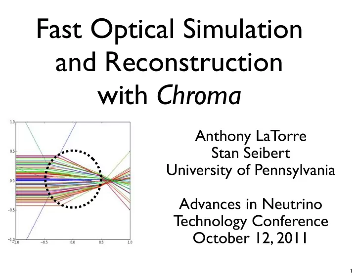
Anthony LaTorre Stan Seibert University of Pennsylvania Advances in Neutrino Technology Conference October 12, 2011
1
Fast Optical Simulation and Reconstruction with Chroma Anthony - - PowerPoint PPT Presentation
Fast Optical Simulation and Reconstruction with Chroma Anthony LaTorre Stan Seibert University of Pennsylvania Advances in Neutrino Technology Conference October 12, 2011 1 Two Ideas (+URL) A sufficiently fast and accurate Monte Carlo is
1
2
We use the ML method all the time.
Hard part: Creating the PDFs for all of
5 10 15 0.5 1 0.5 1
1
3
Typical technique:
Cut all the hard to model / “low” information data.
(Ex: late scattered photons)
Make analytic approximations to detector geometry
and physics processes.
Integrate over internal degrees of freedom.
P S
i = λNorm
λ2
λ1
dλ λ2 P s
1 × P s 2 × P s 3 × P s 4 × P s 5 × P s 6
ρscat
i
= 1 V
2π
i sin θ r2 drdθdφ
4
If you have a Monte Carlo that reproduces the real
In the limit of infinite CPU processing power, for
Very natural to include scattered light, realistic
Easy to track changing detector conditions. If your MC is accurate, then this is the best you could
5
“Analytic” reconstruction algorithms typical work
Monte Carlo based reconstruction is a non-
6
Many experiments use Monte Carlo to create
Ex: SNO and MiniCLEAN have had success with
7
GEANT4 is far too slow, structurally resistant to
A Monte Carlo-derived likelihood has an intrinsic
8
9
10
11
Solid Modeling: Build objects using various 3D
Surface Modeling: Build objects using a surface
12
Bounding Volume Hierarchy: A tree of boxes where each node encloses all of its descendants. Does not need to partition the space and siblings can overlap! Leaf nodes contain list of triangles
13
14
15
16
17
18
19
GEANT4 is slow because of the overhead of
A triangle mesh can reasonably approximate most
Fast mesh techniques are well-studied in the
Plenty of tools for manipulating triangle meshes
20
inside: heavy water
inside: acrylic
21
In GEANT4, the detector is constructed with a
GEANT4’s “voxelization” technique further
In Chroma, the tree is constructed dynamically for
Much more aggressive than voxelization, and can
22
Each event has large numbers of photons. Perfect application for GPU parallelization!
GTX 580
23
24
This is not the Google Chrome logo.
25
This is still not the Google Chrome logo.
Generate PDFs
26
27
Digitize this:
SNO NIM paper
28
photocathode surface glass envelope
To get this:
reflector Note: This is rendered with the actual simulation code!
29
30
31
Speed (outside): 3-10 fps = 1.4M to 4.8M track steps per second CAD model courtesy of Chris Ng 22 million triangles in whole detector Speed (inside): ? fps = ?? M track steps per second
32
33
34
35
Most time consuming part: finding Statue of Liberty STL file and determining scale factor for accurate height. Nearly every CAD program can dump STL files. Quickly add complex shapes to detector without massive performance loss.
36
LBNE candidate 12” PMT + Light Collector in water
37
LBNE candidate 12” PMT + Light Collector in water
37
Chroma propagates only photons (refraction, diffuse
Our Simulation class can spawn multiple GEANT4
If you produce starting photon vertices some other
38
39
40
600 thousand photon vertices per second per
~7 million track segments per second
~3 million photons per second (incl. physics) Requires ~2 GB of GPU memory and ~5 GB of
Ex: 1 GeV electrons = 4.1 events per second
41
generating events with the appropriate distribution of initial photon vertices.
changing “e-” to “mu-” in the generator function.
(e- track histories) vs. fit for (initial particle direction)
integrate over these uninteresting (or unobservable) degrees of freedom.
to fit for the direction of a gamma, rather than integrate over the space of all π0 decays.
42
43
44
45
46
Pi(t) = Z Particle Physics Z Optics Z Detector Response Pi(t) = Z GEANT4 Z Chroma Z DAQ
2M photons/ sec (50 events/sec @ 100 MeV) 3.5M (or 10M) photons/sec (250 events/ sec) 4k events/ sec
47
from ¡chroma ¡import ¡Simulation, ¡Likelihood, ¡\ ¡ ¡ ¡ ¡ ¡ ¡ ¡ ¡constant_particle_gun import ¡chroma.demo from ¡itertools ¡import ¡islice import ¡numpy ¡as ¡np detector ¡= ¡chroma.demo.detector() sim ¡= ¡Simulation(detector) gen ¡= ¡constant_particle_gun('e-‑', ¡ ¡ ¡ ¡ ¡ ¡ ¡ ¡ ¡ ¡ ¡ ¡ ¡ ¡ ¡ ¡ ¡ ¡ ¡ ¡ ¡ ¡ ¡ ¡ ¡ ¡ ¡ ¡pos=(0,0,0), ¡ ¡ ¡ ¡ ¡ ¡ ¡ ¡ ¡ ¡ ¡ ¡ ¡ ¡ ¡ ¡ ¡ ¡ ¡ ¡ ¡ ¡ ¡ ¡ ¡ ¡ ¡ ¡dir=(1,0,0), ¡ ¡ ¡ ¡ ¡ ¡ ¡ ¡ ¡ ¡ ¡ ¡ ¡ ¡ ¡ ¡ ¡ ¡ ¡ ¡ ¡ ¡ ¡ ¡ ¡ ¡ ¡ ¡ke=100) event ¡= ¡sim.simulate(islice(gen,1)).next() likelihood ¡= ¡Likelihood(sim, ¡event)
48
for ¡x ¡in ¡np.linspace(-‑1.0, ¡1.0, ¡20): ¡ ¡ ¡ ¡hypothesis ¡= ¡constant_particle_gun('e-‑', ¡ ¡ ¡ ¡ ¡ ¡ ¡ ¡ ¡ ¡ ¡ ¡ ¡ ¡ ¡ ¡ ¡ ¡ ¡ ¡ ¡ ¡ ¡ ¡ ¡ ¡ ¡ ¡ ¡ ¡ ¡ ¡ ¡ ¡ ¡ ¡ ¡ ¡ ¡pos=(x,0,0), ¡ ¡ ¡ ¡ ¡ ¡ ¡ ¡ ¡ ¡ ¡ ¡ ¡ ¡ ¡ ¡ ¡ ¡ ¡ ¡ ¡ ¡ ¡ ¡ ¡ ¡ ¡ ¡ ¡ ¡ ¡ ¡ ¡ ¡ ¡ ¡ ¡ ¡ ¡dir=(1,0,0), ¡ ¡ ¡ ¡ ¡ ¡ ¡ ¡ ¡ ¡ ¡ ¡ ¡ ¡ ¡ ¡ ¡ ¡ ¡ ¡ ¡ ¡ ¡ ¡ ¡ ¡ ¡ ¡ ¡ ¡ ¡ ¡ ¡ ¡ ¡ ¡ ¡ ¡ ¡ke=100) ¡ ¡ ¡ ¡L ¡= ¡likelihood.eval(hypothesis, ¡neval=800, ¡ ¡ ¡ ¡ ¡ ¡ ¡ ¡ ¡ ¡ ¡ ¡ ¡ ¡ ¡ ¡ ¡ ¡ ¡ ¡ ¡ ¡ ¡ ¡ ¡nreps=4, ¡ndaq=32) ¡ ¡ ¡ ¡print ¡x, ¡L
49
50
Photon propagation core is mostly stable, but always
Add re-emission of absorbed photons Understand how best to leverage Monte Carlo output
Refine our strategy (not in this talk) for minimization
Do some likelihood maximization!
51
52
53