FE Review-Transportation 1 FE Review-Transportation 2 FE - - PDF document

FE Review-Transportation 1

FE Review-Transportation 2

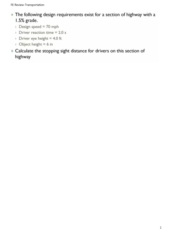
FE Review-Transportation 3

FE Review-Transportation 4

FE Review-Transportation 5

FE Review-Transportation 6

FE Review-Transportation 7

FE Review-Transportation 8

FE Review-Transportation 9

FE Review-Transportation 10

FE Review-Transportation 11

FE Review-Transportation 12

FE Review-Transportation 13

FE Review-Transportation 14

FE Review-Transportation 15

FE Review-Transportation 16

FE Review-Transportation 17

• 1. An interstate weigh station can weigh an average of

20 trucks per hour. Trucks arrive at the average rate of 12 trucks per hour. Performance is described by an

M/ M/1 model. What is most nearly the steady-state

value of the trucks' time spent waiting to be weighed? (A) 0.13 hr/truck

(B) 0.25 hr/truck

(C) 4.0 hr/truck (D) 8.0 hr/truck

• 2. A traffic flow relationship is given by q= kv, where q

is the traffic volume in veh/hr, k is the traffic density in veh/mi, and v is the mean speed in mi/hr. The mean speed on a road in mi/hr is given by the relationship

V = 60 mi - (o.2

~)

k hr veh-hr The maximum capacity of overall traffic volume for this road is most nearly (A) 3400 veh/hr (B) 4300 veh/hr (C) 4500 veh/hr (D) 5000 veh/hr

• 3. A highway weigh station can inspect an average of

16 trucks per hour. Trucks arrive at the average rate of 10 trucks per hour. Performance is described by an

M/ M/1 model. What is most nearly the steady-state

value of the number of trucks in the station? (A) 0.16

t,l'\ i,.,u

(B) 0.60 (C) 1.7 (D) 2.5 FE Review-Transportation 18

• 4. Vehicles arrive at a parking garage at an average rate
• f 45 vehicles per hour. Vehicles are parked by either of

two attendants at an average rate of one vehicle per minute for each attendant. The queue discipline is first come, first served. The arrival of vehicles is modeled as a Poisson's distribution and attendant parking time is modeled as an exponential distribution. What is most nearly the probability that at least one attendant will be idle?

(A) 0.34 (B) 0.45 (C) 0.52 (D) 0.80

• 5. The relationship between traffic density and mean

vehicle speed is shown for a particular road.

>

• a

Q) Q)

Cl.

(/) Q)

~ .c

Q)

>

C

Ctl Q)

E 60 53 50 40 30 20 10

10

20 30 40 50

traffic density, k (veh/mi)

60 70 66.25

What is most nearly the maximum traffic volume for this road? (A) 760 veh/hr (B) 880 veh/hr (C) 900 veh/hr (D) 960 veh/hr FE Review-Transportation 19

• 6. A border's point of entry can weigh an average of

24 trucks per hour. Trucks arrive at the average rate of 15 trucks per hour. Performance is described by an

M/ M/1 model. What is most nearly the steady-state

value of the probability that there will be five trucks being weighed or waiting to be weighed at any time? (A) 0.010 (B) 0.036 (C) 0.38 (D) 0.63

• 1. Boundary and traverse lines bounding an irregular

area are shown.

boundary. 34 ft I

31 ft1 29 ft 23 ft I 21 ft I 23 ft i

traverse 30 ft line 30 ft 30 ft 30 ft 30 ft

The total area between the irregular boundary and the traverse line is most nearly (A) 3600 ft2 (B) 3800 ft2 (C) 4000 ft2 (D) 4200 ft2 FE Review-Transportation 20

• 2. Global positioning system (GPS) latitudes and long­

itudes were taken of a plot of land. In the region where the plot is located, the length of a degree of latitude is 364,320 ft, and the length of a degree of longitude is

248,160 ft.

N 47.3116° E 122.8163°

Br

N 47.3118° E 122.8184°

C

• C\l

CO CD

00

N 47.3105° E 122.8162° D N 47.3104° E 122.8183°

1°E/248,160 ft •

What is most nearly the area of the plot? (A) 5.0 ac (B) 5.1 ac (C) 5.3 ac (D) 5.4 ac

• 3. The illustration shows a curve from x = 0 to x = 6.

4

Using intervals of 1, what is most nearly the area under the curve predicted by Simpson's l/z rule? (A) 14 (B) 15 (C) 16 (D) 17 FE Review-Transportation 21

• 4. A polygon is created by enclosing lines as shown.

C

"-—J?

A E 1 G 2

Using an interval of 1, what is most nearly the area of the polygon predicted by the trapezoidal rule? (A) 15 (B) 16 (C) 17 (D) 18

• 5. Which statement(s) concerning methods used to

determine areas under a curve or line is/are true? I. The trapezoidal rule applies to areas where the irregular sides are curved. II. Simpson's rule only applies to an odd number of data points. III. The area by coordinates method can be used if the coordinates of the traverse leg end points are known. (A) I only (B) III only (C) I and III (D) I, II, and III FE Review-Transportation 22

• 1. A horizontal curve is laid out with the point of curve,

PC, station and the length of long chord, LC, as shown.

PT I = 104 36' /

/

sta 10 + 46 b

PC I---

The radius of the curve is most nearly (A) 520 ft

(B) 560 ft (C) 620 ft (D) 670 ft

• 2. A freeway route has a horizontal curve with a PI at

sta 11+01.86, an intersection angle, I, of 12°24'00" right, and a radius of 1760 ft. The PC is located at

(A) sta 9+10 (B) sta 9+22 (C) sta 10+11 (D) sta 10+24 FE Review-Transportation 23

• 3. A vertical sag curve has a length of 8 sta and con­

nects a —2.0% grade to a 1.6% vertical grade. The PVI is located at sta 87+00 and has an elevation of 2438 ft.

L = 8 sta

PVC PVT 2.0% 1.6% PVI = sta 87 +

00 PVI elevation = 2438 ft

The elevation of the lowest point on the vertical curve is most nearly (A) 2420 ft (B) 2430 ft (C) 2440 ft (D) 2450 ft FE Review-Transportation 24

• 4. A 6° curve has forward and back tangents that inter­

sect at sta 14+87.33.

PI at sta 14+87.33

1= 11°21

'35"

PC

The station of the point of curve, PC, is most nearly (A) sta 5+32

(B) sta 9+93 (C) sta 11+28 (D) sta 13+92 FE Review-Transportation 25