[PPT] - Fundamentals of Signals Overview Equation for a line Definition x ( PowerPoint Presentation

SLIDE 1

Examples of Signals Definition: an abstraction of any measurable quantity that is a function of one or more independent variables such as time or space. Examples:

A voltage in a circuit
A current in a circuit
The Dow Jones Industrial average
Electrocardiograms
A sin(ωt + φ)
Speech/music
Force exerted on a shock absorber
Concentration of Chlorine in a water supply
J. McNames

Portland State University ECE 222 Signal Fundamentals

Ver. 1.15

3

Fundamentals of Signals Overview

Definition
Examples
Energy and power
Signal transformations
Periodic signals
Symmetry
Exponential & sinusoidal signals
Basis functions
J. McNames

Portland State University ECE 222 Signal Fundamentals

Ver. 1.15

1

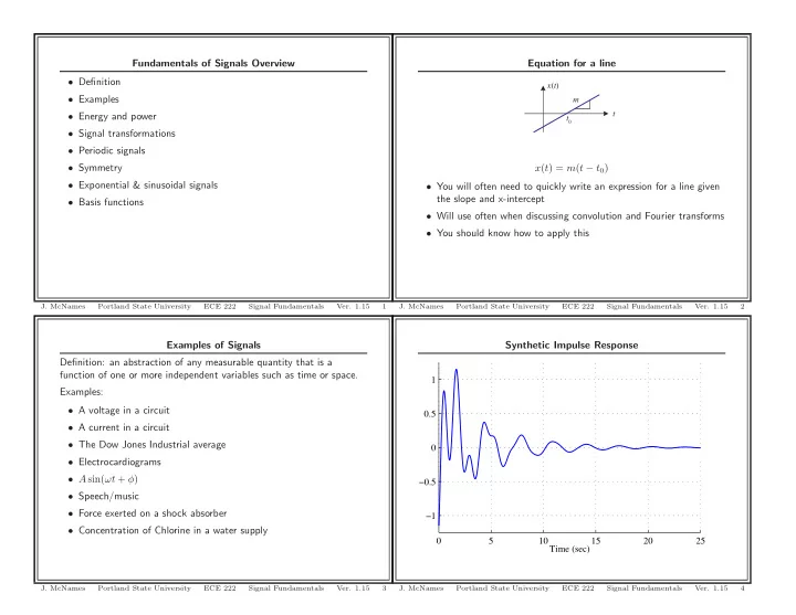
Synthetic Impulse Response

5 10 15 20 25 −1 −0.5 0.5 1 Time (sec)

J. McNames

Portland State University ECE 222 Signal Fundamentals

Ver. 1.15

4

Equation for a line

t t0 m x(t)

x(t) = m(t − t0)

You will often need to quickly write an expression for a line given

the slope and x-intercept

Will use often when discussing convolution and Fourier transforms
You should know how to apply this
J. McNames

Portland State University ECE 222 Signal Fundamentals

Ver. 1.15

2

SLIDE 2

Arterial Blood Pressure

0.5 1 1.5 2 2.5 60 70 80 90 100 110 120 Time (sec) ABP (mmHg)

J. McNames

Portland State University ECE 222 Signal Fundamentals

Ver. 1.15

7

Microelectrode Recording

2 2.01 2.02 2.03 2.04 2.05 2.06 −0.6 −0.4 −0.2 0.2 0.4 0.6 0.8 Time (sec)

J. McNames

Portland State University ECE 222 Signal Fundamentals

Ver. 1.15

5

Speech

1.2 1.25 1.3 1.35 1.4 1.45 1.5 1.55 1.6 1.65 −0.4 −0.3 −0.2 −0.1 0.1 0.2 0.3 0.4 Time (sec) Linus: Philosophy of Wet Suckers

J. McNames

Portland State University ECE 222 Signal Fundamentals

Ver. 1.15

8

Electrocardiogram

0.5 1 1.5 2 2.5 6.5 7 7.5 8 8.5 Time (sec)

J. McNames

Portland State University ECE 222 Signal Fundamentals

Ver. 1.15

6

SLIDE 3

Signal Energy & Power

For most of this class we will use a broad definition of power and

energy that applies to any signal x(t) or x[n]

Instantaneous signal power

P(t) = |x(t)|2 P[n] = |x[n]|2

Signal energy

E(t0, t1) = t1

t0

|x(t)|2 dt E(n0, n1) =

n1

n=n0

|x[n]|2

Average signal power

P(t0, t1) = 1 t1 − t0 t1

t0

|x(t)|2 dt P(n0, n1) = 1 n1 − n0 + 1

n1

n=n0

|x[n]|2

J. McNames

Portland State University ECE 222 Signal Fundamentals

Ver. 1.15

11

Chaos

50 100 150 200 250 300 350 400 450 −15 −10 −5 5 10 15 Time (samples)

J. McNames

Portland State University ECE 222 Signal Fundamentals

Ver. 1.15

9

Signal Energy & Power Comments Usually, the limits are taken over an infinite time interval E∞ = ∞

−∞

|x(t)|2 dt E∞ =

∞

n=−∞

|x[n]|2 P∞ = lim

T →∞

1 2T T

−T

|x(t)|2 dt P∞ = lim

N→∞

1 2N + 1

N

n=−N

|x[n]|2

We will encounter many types of signals
Some have infinite average power, energy, or both
A signal is called an energy signal if E∞ < ∞
A signal is called a power signal if 0 < P∞ < ∞
A signal can be an energy signal, a power signal, or neither type
A signal can not be both an energy signal and a power signal
J. McNames

Portland State University ECE 222 Signal Fundamentals

Ver. 1.15

12

Discrete-time & Continuous-time

We will work with both types of signals
Continuous-time signals

– Will always be treated as a function of t – Parentheses will be used to denote continuous-time functions – Example: x(t) – t is a continuous independent variable (real-valued)

Discrete-time signals

– Will always be treated as a function of n – Square brackets will be used to denote discrete-time functions – Example: x[n] – n is an independent integer

J. McNames

Portland State University ECE 222 Signal Fundamentals

Ver. 1.15

10

SLIDE 4

Example 1: Workspace (2)

J. McNames

Portland State University ECE 222 Signal Fundamentals

Ver. 1.15

15

Example 1: Energy & Power Determine whether the energy and average power of each of the following signals is finite. x(t) =

8

|t| < 5

therwise

x[n] = j x[n] = A cos(ωn + φ) x(t) =

eat

t > 0

therwise

x[n] = ejωn

J. McNames

Portland State University ECE 222 Signal Fundamentals

Ver. 1.15

13

Signal Energy & Power Tips

There are a few rules that can help you determine whether a

signal has finite energy and average power

Signals with finite energy have zero average power:

E∞ < ∞ ⇒ P∞ = 0

Signals of finite duration and amplitude have finite energy:

x(t) = 0 for |t| > c ⇒ E∞ < ∞

Signals with finite average power have infinite energy:

P∞ > 0 ⇒ E∞ = ∞

J. McNames

Portland State University ECE 222 Signal Fundamentals

Ver. 1.15

16

Example 1: Workspace (1)

J. McNames

Portland State University ECE 222 Signal Fundamentals

Ver. 1.15

14

SLIDE 5

Example 2: Axes for x(t + 2) & x( t

2)

x(t)

1 1 2 3 4

1
1
2
3
4

t t

1 1 2 3 4

1
1
2
3
4

t

1 1 2 3 4

1
1
2
3
4
J. McNames

Portland State University ECE 222 Signal Fundamentals

Ver. 1.15

19

Signal Transformations

Time shift: x(t − t0) and x[n − n0]

– If t0 > 0 or n0 > 0, signal is shifted to the right – If t0 < 0 or n0 < 0, signal is shifted to the left

Time reversal: x(−t) and x[−n]
Time scaling: x(αt) and x[αn]

– If α > 1, signal appears compressed – If 1 > α > 0, signal appears stretched

J. McNames

Portland State University ECE 222 Signal Fundamentals

Ver. 1.15

17

Example 2: Axes for x(2t) & x(2 − 2t)

x(t)

1 1 2 3 4

1
1
2
3
4

t t

1 1 2 3 4

1
1
2
3
4

t

1 1 2 3 4

1
1
2
3
4
J. McNames

Portland State University ECE 222 Signal Fundamentals

Ver. 1.15

20

Example 2: Signal Transformations

x(t)

1 1 2 3 4

1
1
2
3
4

t t

1 1 2 3 4

1
1
2
3
4

t

1 1 2 3 4

1
1
2
3
4

Use the signal shown above to draw the following: x(−t), x(t − 1), x(t + 2), x( t

2), x(2t), x(2 − 2t).

J. McNames

Portland State University ECE 222 Signal Fundamentals

Ver. 1.15

18

SLIDE 6

Example 4: Odd Symmetry

x(t)

1 1 2 3 4

1
1
2
3
4

t t

1 1 2 3 4

1
1
2
3
4

t

1 1 2 3 4

1
1
2
3
4

Draw the odd component of the signal shown above.

J. McNames

Portland State University ECE 222 Signal Fundamentals

Ver. 1.15

23

Even & Odd Symmetry xe(t) =

1 2 (x(t) + x(−t))

xo(t) =

1 2 (x(t) − x(−t))

x(t) = xe(t) + xo(t)

The symmetry of a signal under time reversal will be useful later

when we discuss transforms

A signal is even if and only if x(t) = x(−t)
A signal is odd if and only if x(t) = −x(−t)
cos(kω0t) is an even signal
sin(kω0t) is an odd signal
Any signal can be written as the sum of an odd signal and an even

signal

J. McNames

Portland State University ECE 222 Signal Fundamentals

Ver. 1.15

21

Example 5: Even & Odd Symmetry

t

1 1 2 3 4

1
1
2
3
4

t

1 1 2 3 4

1
1
2
3
4

t

1 1 2 3 4

1
1
2
3
4

Show that the sum of the even and odd components of the signal is equal to the original signal graphically.

J. McNames

Portland State University ECE 222 Signal Fundamentals

Ver. 1.15

24

Example 3: Even Symmetry

x(t)

1 1 2 3 4

1
1
2
3
4

t t

1 1 2 3 4

1
1
2
3
4

t

1 1 2 3 4

1
1
2
3
4

Draw the even component of the signal shown above.

J. McNames

Portland State University ECE 222 Signal Fundamentals

Ver. 1.15

22

SLIDE 7

Example 6: Aean, A = 1 and a = ± 1

5

−10 −5 5 10 15 20 25 30 200 400 600 −10 −5 5 10 15 20 25 30 2 4 6 8 Time (n)

J. McNames

Portland State University ECE 222 Signal Fundamentals

Ver. 1.15

27

Periodic Signals A signal is periodic if there is a positive value of T or N such that x(t) = x(t + T) x[n] = x[n + N]

The fundamental period,T0, for continuous-time signals is the

smallest positive value of T such that x(t) = x(t + T)

The fundamental period,N0, for discrete-time signals is the

smallest positive integer of N such that x[n] = x[n + N]

Signals that are not periodic are said to be aperiodic
J. McNames

Portland State University ECE 222 Signal Fundamentals

Ver. 1.15

25

Example 6: MATLAB Code

n = -10:30; % Time index subplot(2,1,1); y = exp(n/5); % Growing exponential h = stem(n,y); set(h(1),’Marker’,’.’); set(gca,’Box’,’Off’); subplot(2,1,2); y = exp(-n/5); % Decaying exponential h = stem(n,y); set(h(1),’Marker’,’.’); set(gca,’Box’,’Off’); xlabel(’Time (n)’);

J. McNames

Portland State University ECE 222 Signal Fundamentals

Ver. 1.15

28

Exponential and Sinusoidal Signals Exponential signals x(t) = Aeat x[n] = Aean where A and a are complex numbers.

Exponential and sinusoidal signals arise naturally in the analysis of

linear systems

Example: simple harmonic motion that you learned in physics
There are several distinct types of exponential signals

– A and a real – A and a imaginary – A and a complex (most general case)

J. McNames

Portland State University ECE 222 Signal Fundamentals

Ver. 1.15

26

SLIDE 8

Example 7: MATLAB Code

fs = 500; % Sample rate (Hz) t = -10:1/fs:30; % Time index (s) a = j; A = 1; y = Aexp(at); h = plot3(t,imag(y),real(y),’b’); hold on; h = plot3(t,ones(size(t)),real(y),’r’); h = plot3(t,imag(y),-ones(size(t)),’g’); hold off; grid on; xlabel(’Time (s)’); ylabel(’Imaginary Part’); zlabel(’Real Part’); title(’Complex:Blue Real:Red Imaginary:Green’); view(27.5,22);

J. McNames

Portland State University ECE 222 Signal Fundamentals

Ver. 1.15

31

Sinusoidal Exponential Signal Comments x(t) = Aeat = A(ea)t = Aαt x[n] = Aean = A(ea)n = Aαn When a is imaginary, then Euler’s equation applies: ejωt = cos(ωt) + j sin(ωt) ejωn = cos(ωn) + j sin(ωn)

Since |ejωt| = 1, this looks like a coil in a plot of the complex

plane versus time

ejωt is Periodic with fundamental period T = 2π

ω

Real part is sinusoidal: Re{Aejωt} = A cos(ωt)
Imaginary part is sinusoidal: Im{Aejωt} = A sin(ωt)
These signals have infinite energy, but finite (constant) average

power, P∞

J. McNames

Portland State University ECE 222 Signal Fundamentals

Ver. 1.15

29

Sinusoidal Exponential Harmonics

In order for ejωt to be periodic with period T, we require that

ejωt = ejω(t+T ) = ejωtejωT for all t

This implies ejωT = 1 and therefore

ωT = 2πk where k = 0, ±1, ±2, . . .

There is more than one frequency ω that satisfies the constraint

x(t) = x(t + T) where T = 2πk

ω

The fundamental frequency is given by k = 1:

ω0 = 2π T0

The other frequencies that satisfy this constraint are then integer

multiples of ω0

J. McNames

Portland State University ECE 222 Signal Fundamentals

Ver. 1.15

32

Example 7: Aeat, A = 1 and a = j

−10 10 20 30 −1 1 −1 −0.5 0.5 1 Imaginary Part Complex:Blue Real:Red Imaginary:Green Time (s) Real Part

J. McNames

Portland State University ECE 222 Signal Fundamentals

Ver. 1.15

30

SLIDE 9

Example 9: Discrete-Time Harmonics

−1 1 φ0 −1 1 φ1 −1 1 φ2 −1 1 φ3 −10 −5 5 10 15 20 25 30 35 40 −1 1 φ4 Time (n)

J. McNames

Portland State University ECE 222 Signal Fundamentals

Ver. 1.15

35

Sinusoidal Exponential Harmonics Continued A harmonically related set of complex exponentials is a set of exponentials with fundamental frequencies that are all multiples of a single positive frequency ω0 φk(t) = ejkω0t where k = 0, ±1, ±2, . . .

For k = 0, φk(t) is a constant
For all other values φk(t) is periodic with fundamental frequency

|k|ω0

This is consistent with how the term harmonic is used in music
Sinusoidal harmonics will play a very important role when we

discuss Fourier series and periodic signals

J. McNames

Portland State University ECE 222 Signal Fundamentals

Ver. 1.15

33

Example 9: MATLAB Code

n = -10:40; % Time index

mega = 2*pi/20;

% Frequency (radians/sample) N = 4; for cnt = 0:N, subplot(N+1,1,cnt+1); phi = exp(j*cnt*omega*n); h = stem(n,real(phi)); set([h(1)],’Marker’,’.’); ylim([-1.1 1.1]); ylabel(sprintf(’\\phi_%d’,cnt)); set(gca,’YGrid’,’On’) if cnt~=N, set(gca,’XTickLabel’,[]); end; end; xlabel(’Time (n)’); figure; t = -10:0.01:40; % Time index

mega = 0.05*2*pi;

% Frequency (radians/sec) - 0.05 Hz N = 4; for cnt = 0:N, subplot(N+1,1,cnt+1); phi = exp(j*cnt*omega*t); h = plot(t,real(phi)); ylim([-1.1 1.1]); ylabel(sprintf(’\\phi_%d’,cnt)); grid on; if cnt~=N, set(gca,’XTickLabel’,[]); end; end; xlabel(’Time (s)’);

J. McNames

Portland State University ECE 222 Signal Fundamentals

Ver. 1.15

36

Example 8: Continuous-Time Harmonics

−1 1 φ0 −1 1 φ1 −1 1 φ2 −1 1 φ3 −10 −5 5 10 15 20 25 30 35 40 −1 1 φ4 Time (s)

J. McNames

Portland State University ECE 222 Signal Fundamentals

Ver. 1.15

34

SLIDE 10

Example 10: MATLAB Code

n = -10:40; % Time index C = 1; subplot(2,1,1); a = 0.1 + j*0.5; y = real(C*exp(a*n)); % Growing exponential t = min(n):0.1:max(n); h = plot(t, real(C*exp(real(a)*t)),t,-real(C*exp(real(a)*t))); set(h,’Color’,[0.5 0.5 0.5]); hold on; h = stem(n,y); set(h(1),’Marker’,’.’); hold off; box off; grid on; ylim([-50 50]); ylabel(’Real Part’); subplot(2,1,2); a = -0.1 + j*0.5; y = real(C*exp(a*n)); % Growing exponential t = min(n):0.1:max(n); h = plot(t, real(C*exp(real(a)*t)),t,-real(C*exp(real(a)*t))); set(h,’Color’,[0.5 0.5 0.5]); hold on; h = stem(n,y); set(h(1),’Marker’,’.’); hold off; box off; grid on; ylim([-2 2]); xlabel(’Time (n)’); ylabel(’Real Part’);

J. McNames

Portland State University ECE 222 Signal Fundamentals

Ver. 1.15

39

Damped Complex Sinusoidal Exponentials x(t) = Aeat x[n] = Aean

When a is complex, these become damped sinusoidal exponentials
Let a = α + jω. Then

x(t) = Aeat = (Aeαt) × ejωt x[n] = Aean = (Aeαn) × ejωn

Thus, these are equivalent to multiplying an complex sinusoid by a

real exponential

J. McNames

Portland State University ECE 222 Signal Fundamentals

Ver. 1.15

37

Example 11: Aeat, A = 1 and a = ±0.05 + j2

−10 10 20 30 −2 2 −2 2 Imaginary Part Complex:Blue Real:Red Imaginary:Green Real Part −10 10 20 30 −2 2 −2 2 Imaginary Part Time (s) Real Part

J. McNames

Portland State University ECE 222 Signal Fundamentals

Ver. 1.15

40

Example 10: Aean, A = 1 and a = ±0.1 + j0.5

−10 −5 5 10 15 20 25 30 35 40 −50 50 Real Part −10 −5 5 10 15 20 25 30 35 40 −2 −1 1 2 Time (n) Real Part

J. McNames

Portland State University ECE 222 Signal Fundamentals

Ver. 1.15

38

SLIDE 11

Discrete-Time Unit Step

n

1

The discrete-time unit step is defined as u[n] =

0,

n < 0 1, n ≥ 0

J. McNames

Portland State University ECE 222 Signal Fundamentals

Ver. 1.15

43

Example 11: MATLAB Code

fs = 500; % Sample rate (Hz) t = -10:1/fs:30; % Time index (s) subplot(2,1,1); a = -0.05 + j*2; y = C*exp(a*t); h = plot3(t,imag(y),real(y),’b’); hold on; h = plot3(t,2*ones(size(t)),real(y),’r’); h = plot3(t,imag(y),-2*ones(size(t)),’g’); hold off; grid on; ylabel(’Imaginary Part’); zlabel(’Real Part’); title(’Complex:Blue Real:Red Imaginary:Green’); axis([min(t) max(t) -2 2 -2 2]); view(27.5,22); subplot(2,1,2); a = +0.05 + j*2; y = C*exp(a*t); h = plot3(t,imag(y),real(y),’b’); hold on; h = plot3(t,2*ones(size(t)),real(y),’r’); h = plot3(t,imag(y),-2*ones(size(t)),’g’); hold off; grid on; xlabel(’Time (s)’); ylabel(’Imaginary Part’); zlabel(’Real Part’); axis([min(t) max(t) -2 2 -2 2]); view(27.5,22);

J. McNames

Portland State University ECE 222 Signal Fundamentals

Ver. 1.15

41

Discrete-Time Basis Functions

There is a close relationship between δ[n] and u[n]

δ[n] = u[n] − u[n − 1] u[n] =

n

k=−∞

δ[k] u[n] =

∞

k=0

δ[n − k]

The unit impulse can be used to sample a discrete-time signal

x[n]: x[0] =

∞

k=−∞

x[k]δ[k] x[n] =

∞

k=−∞

x[k]δ[n − k]

This ability to use the unit impulse to extract a single value of x[n]

through multiplication will play an important role later in the term

J. McNames

Portland State University ECE 222 Signal Fundamentals

Ver. 1.15

44

Discrete-Time Unit Impulse

n

1

The discrete-time unit impulse is defined as δ[n] =

0,

n = 0 1, n = 0

Sometimes called the unit sample
Also called the Kroneker delta
Note that δ[n] has even symmetry so δ[n] = δ[−n]
J. McNames

Portland State University ECE 222 Signal Fundamentals

Ver. 1.15

42

SLIDE 12

Continuous-Time Unit Impulse

t ue(t) t

e

e

e

e t u(t) t 1 1

δe(t) δ(t)

δe(t) due(t)

dt

As e → 0 ,

– ue(t) → u(t) – δe(t) for t = 0 becomes very large – δe(t) for t = 0 becomes zero

δ(t) lime→0 δe(t)
J. McNames

Portland State University ECE 222 Signal Fundamentals

Ver. 1.15

47

Continuous-Time Unit Step

t u(t) 1

u(t)

t < 0

1 t > 0

Sometimes known as the Heaviside function
Discontinuous at t = 0
u(0) is not defined
Not of consequence because it is undefined for an infinitesimal

period of time

J. McNames

Portland State University ECE 222 Signal Fundamentals

Ver. 1.15

45

Continuous-Time Unit Impulse Continued

t 1

δ(t)

t = 0

∞ t = 0 e

−e

δ(t) dt = 1 for any e > 0

Also known as the Dirac delta function
Is zero everywhere except zero
The impulse integral serves as a measure of the impulse amplitude
Drawn as an arrow with unit height
5δ(t) would be drawn as an arrow with height of 5
J. McNames

Portland State University ECE 222 Signal Fundamentals

Ver. 1.15

48

Unit Step for Switches

vs Linear Circuit t=0 vsu(t) Linear Circuit Linear Circuit t=0 is isu(t) Linear Circuit

u(t) useful for representing the opening or closing of switches
We will often solve for or be given initial conditions at t = 0
We can then represent independent sources as though they were

immediately applied at t = 0. More later.

J. McNames

Portland State University ECE 222 Signal Fundamentals

Ver. 1.15

46

SLIDE 13

Unit Impulse Sampling Property +∞

−∞

x(t)δ(t) dt = +∞

−∞

x(0)δ(t) dt = x(0) +∞

−∞

δ(t) dt = x(0) Similarly, +∞

−∞

x(t)δ(t − t0) dt = +∞

−∞

x(t0)δ(t − t0) dt = x(t0) +∞

−∞

δ(t − t0) dt = x(t0)

J. McNames

Portland State University ECE 222 Signal Fundamentals

Ver. 1.15

51

Continuous-Time Unit Impulse Comments δ(t) =

t = 0

∞ t = 0

The impulse should be viewed as an idealization
Real systems with finite inertia do not respond instantaneously
The most important property of an impulse is its area
Most systems will respond nearly the same to sharp pulses

regardless of their shape - if – They have the same amplitude (area) – Their duration is much briefer than the system’s response

The idealized unit impulse is short enough for any system
J. McNames

Portland State University ECE 222 Signal Fundamentals

Ver. 1.15

49

Unit Impulse Sampling Property x(t) = +∞

−∞

x(τ)δ(τ − t) dτ

This integral does not appear to be useful
It will turn out to be very useful
It states that x(t) can be written as a linear combination of scaled

and shifted unit impulses

This will be a key concept when we discuss convolution next week
J. McNames

Portland State University ECE 222 Signal Fundamentals

Ver. 1.15

52

Unit Impulse Properties δ(t)x(t) = δ(t)x(0) δ(at) = 1 |a|δ(t) δ(−t) = δ(t) δ(t) = du(t) dt u(t) = t

−∞

δ(τ) dτ

J. McNames

Portland State University ECE 222 Signal Fundamentals

Ver. 1.15

50