Grid Generation and Refinement Numerical treatment of PDE requires - - PDF document

Scientific Computing I

Module 7: Grid Generation Michael Bader

Lehrstuhl Informatik V

Winter 2005/2006

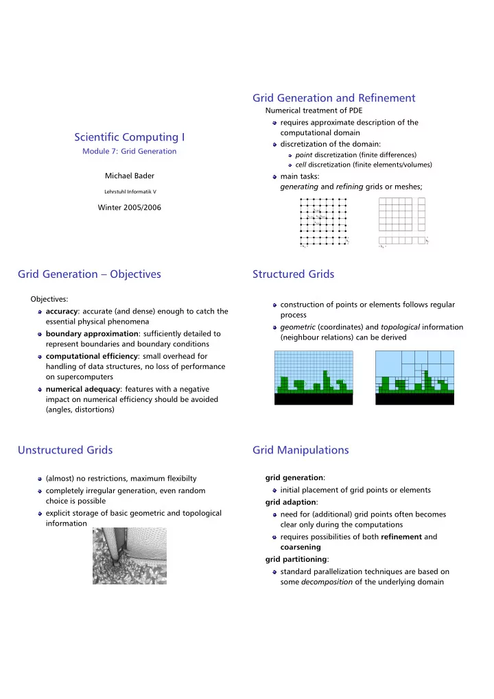
Grid Generation and Refinement

Numerical treatment of PDE requires approximate description of the computational domain discretization of the domain:

point discretization (finite differences) cell discretization (finite elements/volumes)

main tasks: generating and refining grids or meshes;

xi,j xi−1,j xi+1,j xi,j+1 xi,j−1 hx hy hx hy

Grid Generation – Objectives

Objectives: accuracy: accurate (and dense) enough to catch the essential physical phenomena boundary approximation: sufficiently detailed to represent boundaries and boundary conditions computational efficiency: small overhead for handling of data structures, no loss of performance

• n supercomputers

numerical adequacy: features with a negative impact on numerical efficiency should be avoided (angles, distortions)

Structured Grids

construction of points or elements follows regular process geometric (coordinates) and topological information (neighbour relations) can be derived

Unstructured Grids

(almost) no restrictions, maximum flexibilty completely irregular generation, even random choice is possible explicit storage of basic geometric and topological information

Grid Manipulations

grid generation: initial placement of grid points or elements grid adaption: need for (additional) grid points often becomes clear only during the computations requires possibilities of both refinement and coarsening grid partitioning: standard parallelization techniques are based on some decomposition of the underlying domain

Grid Operations

Typical Operations on the Grid: numbering of the nodes/cells

for traversal/processing of the grid for storing the grid for partitioning the grid

identify the neighbours of a node/cell

neighbouring/adjacent nodes/cells/edges due to typical discretization techniques

Regular Structured Grids

rectangular/cartesian grids: rectangles (2D) or cuboids (3D) triangular meshes: triangles (2D) or tetrahedra (3D) row-major or column-major traversal and storage

hx hy

Transformed Structured Grids

transformation of the unit square to the computational domain regular grid is transformed likewise

(0,0) (1,0) (0,1) (1,1) (ξ(0),η(0)) (ξ(1),η(1)) (ξ(0),η(1)) (ξ(1),η(0))

Variants: algebraic: interpolation-based example: Coons patch PDE-based: solve system of PDEs to obtain (ξ(x,y) and η(x,y)

Composite Structured Grids

subdivide (complicated) domain into subdomains of simpler form and use regular meshs on each subdomain at interfaces:

conforming at interface (“glue” required?)

• verlapping grids (chimera grids)

Block Structured Grids

subdivision into logically rectangular subdomains (with logically rectangular local grids) subdomains fit together in an unstructured way, but continuity is ensured (coinciding grid points) popular in computational fluid dynamics

Delauney Triangulation

assume: grid points are already obtained – how to define elements? based on Voronoi diagrams Voronoi region around each given grid point: Vi = {P : P−Pi < P−Pj ∀j = i}

P P P P P P

1 2 3 4 5 6

V V V V V V

1 2 3 4 5 6

Delauney Triangulation (2)

Algorithm

1

Voronoi region around each given grid point: Vi = {P : P−Pi < P−Pj ∀j = i}

2

connect points that are located in adjacent Voronoi regions

3

leads to set of disjoint triangles (tetrahedra in 3D) Applications: closely related to FEM, typically triangles/tetrahedra very widespread

Point Generation

how do we get the grid points? start with a regular grid and refine/modify boundary-based:

start with some boundary point distribution, generate Delaunay triangulation, and subdivide (following suitable rules)

if helpful, add point or lines sources (singularities,

• bound. layers)

Advancing Front methods

Advancing Front Methods

advance a front step-by-step towards interior starting from the boundary (starting front)

P P 1 2 P P P 1 2 P

Advancing Front Methods (2)

Advancing algorithm:

1

choose an edge on the current front, say PQ

2

create a new point R at equal distance d from P and Q

3

determine all grid points lying within a circle around R, radius r

4

• rder these points w.r.t. distance from R

5

for all points, form triangles with P and Q; select one of these triangles

6

add triangle to grid (unless: intersections, . . . )

7

update triangulation and front line: add new cell, update edges

Adaptive Grids

Characterization of adaptive grids: size of grid cells varies considerably to locally improve accuracy sometimes requirement from numerics Challenge for structured grids: efficient storage/traversal retrieve structural information (neighbours, etc.)

Block Adaptive Grids

retain regular structure refinement of entire blocks similar to block structured grids efficient storage and processing but limited w.r.t. adaptivity

Recursively Structured Adaptive Grids

based on recursive subdivision of parent cell(s) leads to tree structures quadtree/octree or substructuring of triangles: efficient storage; flexible adaptivity but complicated processing (recursive algorithms)