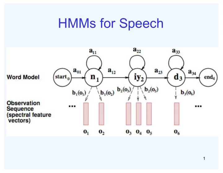
HMMs for Speech 1 Transitions with Bigrams 2 Decoding Finding - - PowerPoint PPT Presentation

hmms for speech
SMART_READER_LITE
LIVE PREVIEW

HMMs for Speech 1 Transitions with Bigrams 2 Decoding Finding - - PowerPoint PPT Presentation

HMMs for Speech 1 Transitions with Bigrams 2 Decoding Finding the words given the acoustics is an HMM inference problem We want to know which state sequence x 1:T is most likely given the evidence e 1:T : * x argmax p x | e ( )


slide-1
SLIDE 1

HMMs for Speech

1

slide-2
SLIDE 2

Transitions with Bigrams

2

slide-3
SLIDE 3

Decoding

3

  • Finding the words given the acoustics is an HMM

inference problem

  • We want to know which state sequence x1:T is most

likely given the evidence e1:T:

  • From the sequence x, we can simply read off the

words

( ) ( )

1: 1:

* 1: 1: 1: 1: 1:

argmax | argmax ,

T T

T T T x T T x

x p x e p x e = =

slide-4
SLIDE 4

Parameter Estimation

4

  • Estimating the distribution of a random variable
  • Elicitation: ask a human (why is this hard?)
  • Empirically: use training data (learning!)
  • E.g.: for each outcome x, look at the empirical rate of

that value:

  • This is the estimate that maximizes the likelihood of the

data

( ) ( )

count total samples

ML

x p x =

( ) ( )

,

i i

L x p x

θ

θ =∏

( )

1 3

ML

p r =

slide-5
SLIDE 5

Example: Spam Filter

5

  • Input: email
  • Output: spam/ham
  • Setup:
  • Get a large collection of

example emails, each labeled “spam” or “ham”

  • Note: someone has to

hand label all this data!

  • Want to learn to predict

labels of new, future emails

  • Features: the attributes

used to make the ham / spam decision

  • Words: FREE!
  • Text patterns: $dd, CAPS
  • Non-text: senderInContacts
  • ……
slide-6
SLIDE 6

Example: Digit Recognition

6

  • Input: images / pixel grids
  • Output: a digit 0-9
  • Setup:
  • Get a large collection of example

images, each labeled with a digit

  • Note: someone has to hand label

all this data!

  • Want to learn to predict labels of

new, future digit images

  • Features: the attributes used to

make the digit decision

  • Pixels: (6,8) = ON
  • Shape patterns: NumComponents,

AspectRation, NumLoops

  • ……
slide-7
SLIDE 7

A Digit Recognizer

7

  • Input: pixel grids
  • Output: a digit 0-9
slide-8
SLIDE 8
  • Classification
  • Given inputs x, predict labels (classes) y
  • Examples
  • Spam detection. input: documents; classes:

spam/ham

  • OCR. input: images; classes: characters
  • Medical diagnosis. input: symptoms; classes:

diseases

  • Autograder. input: codes; output: grades

8

Classification

slide-9
SLIDE 9

Important Concepts

9

  • Data: labeled instances, e.g. emails marked spam/ham
  • Training set
  • Held out set (we will give examples today)
  • Test set
  • Features: attribute-value pairs that characterize each x
  • Experimentation cycle
  • Learn parameters (e.g. model probabilities) on training set
  • (Tune hyperparameters on held-out set)
  • Compute accuracy of test set
  • Evaluation
  • Accuracy: fraction of instances predicted correctly
  • Overfitting and generalization
  • Want a classifier which does well on test data
  • Overfitting: fitting the training data very closely, but not

generalizing well

slide-10
SLIDE 10

General Naive Bayes

10

  • A general naive Bayes model:
  • We only specify how each feature depends on

the class

  • Total number of parameters is linear in n

Y × F

n

parameters

p Y,F

1Fn

( ) =

p Y

( )

p F

i |Y

( )

i

Y parameters n × Y × F parameters

slide-11
SLIDE 11

General Naive Bayes

11

  • What do we need in order to use naive Bayes?
  • Inference (you know this part)
  • Start with a bunch of conditionals, p(Y) and the p(Fi|Y) tables
  • Use standard inference to compute p(Y|F1…Fn)
  • Nothing new here
  • Learning: Estimates of local conditional probability

tables

  • p(Y), the prior over labels
  • p(Fi|Y) for each feature (evidence variable)
  • These probabilities are collectively called the parameters of

the model and denoted by θ

slide-12
SLIDE 12

Inference for Naive Bayes

12

  • Goal: compute posterior over causes
  • Step 1: get joint probability of causes and evidence
  • Step 2: get probability of evidence
  • Step 3: renormalize

p Y, f1 fn

( ) =

p y1, f1 fn

( )

p y2, f1 fn

( )

 p yk, f1 fn

( )

! " # # # # # # $ % & & & & & &

p y1

( )

p fi | c1

( )

i

p y2

( )

p fi | c2

( )

i

 p yk

( )

p fi | ck

( )

i

" # $ $ $ $ $ $ $ $ % & ' ' ' ' ' ' ' '

p f

1 f n

( )

p Y | f1 fn

( )

divide

slide-13
SLIDE 13

Naive Bayes for Digits

13

  • Simple version:
  • One feature Fij for each grid position <i,j>
  • Possible feature values are on / off, based on whether

intensity is more or less than 0.5 in underlying image

  • Each input maps to a feature vector, e.g.
  • Here: lots of features, each is binary valued
  • Naive Bayes model:

→ F

0,0 = 0 F 0,1 = 0 F 0,2 =1 F 0,3 =1 F 0,4 = 0 F 15,15 = 0

p Y | F

0,0F 15,15

( )∝ p Y ( )

p F

i, j |Y

( )

i, j

slide-14
SLIDE 14
  • p(Y=y)
  • approximated by the frequency of each Y in

training data

  • p(F|Y=y)
  • approximated by the frequency of (y,F)

14

Learning in NB (Without smoothing)

slide-15
SLIDE 15

Examples: CPTs

15

1 0.1 2 0.1 3 0.1 4 0.1 5 0.1 6 0.1 7 0.1 8 0.1 9 0.1 0.1

( )

p Y

( )

3,1

| p F

  • n Y

=

1 0.05 2 0.01 3 0.90 4 0.80 5 0.90 6 0.90 7 0.25 8 0.85 9 0.60 0.80

( )

5,5

| p F

  • n Y

=

1 0.01 2 0.05 3 0.05 4 0.30 5 0.80 6 0.90 7 0.05 8 0.60 9 0.50 0.80

slide-16
SLIDE 16

Example: Spam Filter

16

  • Naive Bayes spam

filter

  • Data:
  • Collection of emails labeled

spam or ham

  • Note: some one has to hand

label all this data!

  • Split into training, held-out,

test sets

  • Classifiers
  • Learn on the training set
  • (Tune it on a held-out set)
  • Test it on new emails
slide-17
SLIDE 17

Naive Bayes for Text

17

  • Bag-of-Words Naive Bayes:
  • Features: Wi is the word at position i
  • Predict unknown class label (spam vs. ham)
  • Each Wi is identically distributed
  • Generative model:
  • Tied distributions and bag-of-words
  • Usually, each variable gets its own conditional

probability distribution p(F|Y)

  • In a bag-of-words model
  • Each position is identically distributed
  • All positions share the same conditional probs p(W|C)

p C,W

1Wn

( ) = p C ( )

p Wi |C

( )

i

Word at position i, not ith word in the dictionary!

slide-18
SLIDE 18

Example: Spam Filtering

18

  • Model:
  • What are the parameters?
  • Where do these tables come from?

p C,W

1Wn

( ) = p C ( )

p Wi |C

( )

i

ham 0.66 spam 0.33

( )

p Y

( )

|spam p W

the 0.0156 to 0.0153 and 0.0115

  • f

0.0095 you 0.0093 a 0.0086 with 0.0080 from 0.0075 …

( )

| ham p W

the 0.0210 to 0.0133

  • f

0.0119 2002 0.0110 with 0.0108 from 0.0107 and 0.0105 a 0.0100 …

slide-19
SLIDE 19

Word p(w|spam) p(w|ham) Σ log p(w|spam) Σ log p(w|ham) (prior) 0.33333 0.66666

  • 1.1
  • 0.4

Gary 0.00002 0.00021

  • 11.8
  • 8.9

would 0.00069 0.00084

  • 19.1
  • 16.0

you 0.00881 0.00304

  • 23.8
  • 21.8

like 0.00086 0.00083

  • 30.9
  • 28.9

to 0.01517 0.01339

  • 35.1
  • 33.2

lose 0.00008 0.00002

  • 44.5
  • 44.0

weight 0.00016 0.00002

  • 53.3
  • 55.0

while 0.00027 0.00027

  • 61.5
  • 63.2

you 0.00881 0.00304

  • 66.2
  • 69.0

sleep 0.00006 0.00001

  • 76.0
  • 80.5

19

Spam example

slide-20
SLIDE 20

Problem with this approach

20

2 wins!!

p(feature, C=2) p(C=2)=0.1 p(on|C=2)=0.8 p(on|C=2)=0.1 p(on|C=2)=0.1 p(on|C=2)=0.01 p(feature, C=3) p(C=3)=0.1 p(on|C=3)=0.8 p(on|C=3)=0.9 p(on|C=3)=0.7 p(on|C=3)=0.0

slide-21
SLIDE 21

Another example

21

  • Posteriors determined by relative probabilities

(odds ratios):

( ) ( )

| ham | spam p W p W

south-west inf nation inf morally inf nicely inf extent inf seriously inf …

( ) ( )

| am | am p W sp p W h

screens inf minute inf guaranteed inf $205.00 inf delivery inf signature inf …

What went wrong here?

slide-22
SLIDE 22

Generalization and Overfitting

22

  • Relative frequency parameters will overfit the training data!
  • Just because we never saw a 3 with pixel (15,15) on during training

doesn’t mean we won’t see it at test time

  • Unlikely that every occurrence of “minute” is 100% spam
  • Unlikely that every occurrence of “seriously” is 100% spam
  • What about all the words that don’t occur in the training set at all?
  • In general, we can’t go around giving unseen events zero probability
  • As an extreme case, imagine using the entire email as the
  • nly feature
  • Would get the training data perfect (if deterministic labeling)
  • Wouldn’t generalize at all
  • Just making the bag-of-words assumption gives us some

generalization, but isn’t enough

  • To generalize better: we need to smooth or regularize the

estimates

slide-23
SLIDE 23

Estimation: Smoothing

23

  • Maximum likelihood estimates:
  • Problems with maximum likelihood estimates:
  • If I flip a coin once, and it’s heads, what’s the estimate for

p(heads)?

  • What if I flip 10 times with 8 heads?
  • What if I flip 10M times with 8M heads?
  • Basic idea:
  • We have some prior expectation about parameters (here,

the probability of heads)

  • Given little evidence, we should skew towards our prior
  • Given a lot of evidence, we should listen to the data

( ) ( )

count total samples

ML

x p x =

( )

1 3

ML

p r =

slide-24
SLIDE 24

Estimation: Laplace Smoothing

24

  • Laplace’s estimate (extended):
  • Pretend you saw every outcome k

extra times

  • What’s Laplace with k=0?
  • k is the strength of the prior
  • Laplace for conditionals:
  • Smooth each condition

independently:

( ) ( ) ( )

,0 ,1 ,100 LAP LAP LAP

p X p X p X = = = pLAP,k x

( )=

c x

( )+ k

N + k X

( ) ( ) ( )

,

, | =

LAP k

c x y k p x y c y k X + +

slide-25
SLIDE 25

Estimation: Linear Smoothing

25

  • In practice, Laplace often performs poorly for p(X|Y):
  • When |X| is very large
  • When |Y| is very large
  • Another option: linear interpolation
  • Also get p(X) from the data
  • Make sure the estimate of p(X|Y) isn’t too different from

p(X)

  • What if α is 0? 1?

pLIN x | y

( )=α p

 x | y

( )+ 1−α ( ) p

 x

( )

slide-26
SLIDE 26

Real NB: Smoothing

26

  • For real classification problems, smoothing is critical
  • New odds ratios:

( ) ( )

| ham | spam p W p W

helvetica 11.4 seems 10.8 group 10.2 ago 8.4 area 8.3 …

( ) ( )

| am | am p W sp p W h

verdana 28.8 Credit 28.4 ORDER 27.2 <FONT> 26.9 money 26.5 …

Do these make more sense?

slide-27
SLIDE 27

Tuning on Held-Out Data

27

  • Now we’ve got two kinds of

unknowns

  • Parameters: the probabilities p(Y|X), p(Y)
  • Hyperparameters, like the amount of

smoothing to do: k,α

  • Where to learn?
  • Learn parameters from training data
  • Must tune hyperparameters on different

data

  • Why?
  • For each value of the hyperparameters,

train and test on the held-out data

  • Choose the best value and do a final test
  • n the test data
slide-28
SLIDE 28

Errors, and What to Do

28

  • Examples of errors
slide-29
SLIDE 29

What to Do About Errors?

29

  • Need more features- words aren’t enough!
  • Have you emailed the sender before?
  • Have 1K other people just gotten the same email?
  • Is the sending information consistent?
  • Is the email in ALL CAPS?
  • Do inline URLs point where they say they point?
  • Does the email address you by (your) name?
  • Can add these information sources as new

variables in the NB model

  • Next class we’ll talk about classifiers that let you

add arbitrary features more easily