
SLIDE 1
x2 x1
z
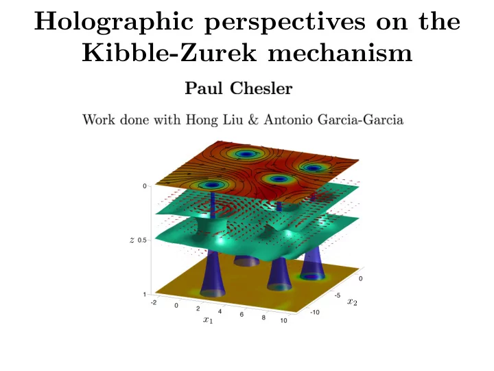
Holographic perspectives on the Kibble-Zurek mechanism z x 2 x 1 - - PowerPoint PPT Presentation
Holographic perspectives on the Kibble-Zurek mechanism z x 2 x 1 What is the Kibble-Zurek mechanism? QFT with 2 nd order phase transition: Example: superfluid Symmetry group U (1) broken for T < T c . broken unbroken Order
x2 x1
z
QFT with 2nd order phase transition:
✏(t) ⌘ 1 T(t) Tc .
n ⇠ ⇠−(d−D).
QFT with 2nd order phase transition:
✏(t) ⌘ 1 T(t) Tc .
n ⇠ ⇠−(d−D).
QFT with 2nd order phase transition:
✏(t) ⌘ 1 T(t) Tc .
n ⇠ ⇠−(d−D).
QFT with 2nd order phase transition:
✏(t) ⌘ 1 T(t) Tc .
n ⇠ ⇠−(d−D).
−tfreeze
+tfreeze
Critical slowing down
∂t
⇒tfreeze ∼ ⌧ νz/(1+νz)
Q
, ⇠freeze ∼ ⌧ ν/(1+νz)
Q
.
nKZ ∼ 1 ⇠d−D
freeze
∼ ⌧ −(d−D)ν/(1+νz)
Q
−tfreeze
+tfreeze
(t) ∼ ✏(t)β
magnitude prediction usually overestimates the real density of defects ob- served in numerics. A better estimate is obtained by using a factor f, to multiply ˆ ξ in the above equations, where f ≈ 5−10 depends on the specific model.29,31–35 Thus, while KZM provides an order-of-magnitude estimate
excerpt from [Del Campo & Zurek]
First holographic study: [Sonner, del Campo, Zurek: two weeks ago]
magnitude prediction usually overestimates the real density of defects ob- served in numerics. A better estimate is obtained by using a factor f, to multiply ˆ ξ in the above equations, where f ≈ 5−10 depends on the specific model.29,31–35 Thus, while KZM provides an order-of-magnitude estimate
excerpt from [Del Campo & Zurek]
Action:
[Hartnoll, Herzog & Horowitz: 0803.3295]
Sgrav = 1 16πGN Z d4x p G R + Λ + 1 q2
, where Λ = 3 and m2 = 2.
– Black-brane solutions with T > Tc have Φ = 0. – Black-brane solutions with T < Tc have Φ 6= 0.
Action:
[Hartnoll, Herzog & Horowitz: 0803.3295]
Sgrav = 1 16πGN Z d4x p G R + Λ + 1 q2
, where Λ = 3 and m2 = 2.
– Black-brane solutions with T > Tc have Φ = 0. – Black-brane solutions with T < Tc have Φ 6= 0.
Game plan:
Action:
[Hartnoll, Herzog & Horowitz: 0803.3295]
Sgrav = 1 16πGN Z d4x p G R + Λ + 1 q2
, where Λ = 3 and m2 = 2.
– Black-brane solutions with T > Tc have Φ = 0. – Black-brane solutions with T < Tc have Φ 6= 0.
T > Tc
Game plan:
Action:
[Hartnoll, Herzog & Horowitz: 0803.3295]
Sgrav = 1 16πGN Z d4x p G R + Λ + 1 q2
, where Λ = 3 and m2 = 2.
– Black-brane solutions with T > Tc have Φ = 0. – Black-brane solutions with T < Tc have Φ 6= 0.
T > Tc
Game plan:
50 100 150 200 250 0.25 0.5 0.75 1
Adiabatic growth |h i|2 ⇠ ✏(t)2β
avg
50 100 150 200 250 0.25 0.5 0.75 1
Adiabatic growth |h i|2 ⇠ ✏(t)2β
avg
50 100 150 200 250 0.25 0.5 0.75 1
Adiabatic growth |h i|2 ⇠ ✏(t)2β
avg
50 100 150 200 250 0.25 0.5 0.75 1
Adiabatic growth |h i|2 ⇠ ✏(t)2β
10
1
10
2
10
3
10 10
1
10
2
tfreeze teq √τQ
avg
C(t, q) = ⇣ Z dt |GR(t, t0, q)|2.
GR(t, t0, q) = ✓(t t0)H(q)ei
R 0t
t dt00!o(✏(t00),q)
where !o is ✏ < 0 quasinormal mode analytically continued to ✏ > 0
Im !o = b✏z⌫ a✏(z2)⌫q2 + O(q4) > 0.
At t > tfreeze, C(t, r) ∼ C0(t)e
−
r2 `co(t)2 ,
where C0(t) ∼ ⇣tfreeze `co(t)−d exp (✓ t tfreeze ◆1+νz) . and `co(t) = ⇠freeze ✓ t tfreeze ◆ 1+(z−2)⌫
2
. Linear response breaks down when C0(t) ∼ ✏(t)2β teq ∼ [log R]
1 1+⌫z tfreeze,
R ∼ ⇣−1⌧
(d−z)⌫−2 1+⌫z
Q
.
At t > tfreeze, C(t, r) ∼ C0(t)e
−
r2 `co(t)2 ,
where C0(t) ∼ ⇣tfreeze `co(t)−d exp (✓ t tfreeze ◆1+νz) . and `co(t) = ⇠freeze ✓ t tfreeze ◆ 1+(z−2)⌫
2
. Linear response breaks down when C0(t) ∼ ✏(t)2β teq ∼ [log R]
1 1+⌫z tfreeze,
R ∼ ⇣−1⌧
(d−z)⌫−2 1+⌫z
Q
.
50 100 150 200 250 0.25 0.5 0.75 1 2 4 6 10
−5
10
−4
10
−3
10
−2
10
−1
10
(t/tfreeze)1+νz
avg
300 600 900 1200 1500 1 1.5 2 2.5 3 tfreeze/√τQ teq /√τQ const. c
c′ √τQ
10
1
10
2
10
3
10 10
1
10
2
tfreeze teq √τQ
For holography (mean field exponents)
1 ζ√τQ and tfreeze ∼ √τQ.
×10−4
t = tfreeze
t = 0.7teq t = 0.85teq
t = teq
If teq tfreeze then
⇣
teq tfreeze
⌘ 1+(z−2)ν
2
⇠freeze.
n/nKZ ⇠ (teq/tfreeze)− (d−D)(1−(z−2)ν)
2
.
teq ⇠ [log N]1/(1+νz)tfreeze.
) Log correction to density of defects n nKZ ⇠ [log τQ]− (d−D)(1+(z−2)ν)
2(1+zν
nKZ.
1 2 3 4 5 0.2 0.4 0.6 0.8 1
t
t/tfreeze
C(t, r)/C(t, r = 0)
1 2 3 4 5 0.2 0.4 0.6 0.8 1
t
t/tfreeze
C(t, r)/C(t, r = 0)
factor of 5!
1 2 3 4 5 0.2 0.4 0.6 0.8 1
t
t/tfreeze
C(t, r)/C(t, r = 0)
factor of 5!
×10−4
t = tfreeze
t = 0.7teq t = 0.85teq
t = teq
10
1
10
2
10
3
10
1
10
2
Nvortices
ξ FW HM
2 τ −1/2
Q
O(25) fewer vortices than KZ estimate
For holography, n ∼ 1 √log N τ −1/2
Q
.
– Initial correlation ξfreeze not imprinted on final state. – Far fewer defects formed than KZ predicts. – Log corrections to KZ scaling law.
0.05 0.1 20 40 60 80
Nvortices ϵf
final