Image Restoration Image Enhancement and Image Restoration both deal - - PowerPoint PPT Presentation

Image Analysis

Image Restoration and Reconstruction Niclas Börlin niclas.borlin@cs.umu.se

Department of Computing Science Umeå University

February 3, 2009

Niclas Börlin (CS, UmU) Image Restoration and Reconstruction February 3, 2009 1 / 31

Image Restoration

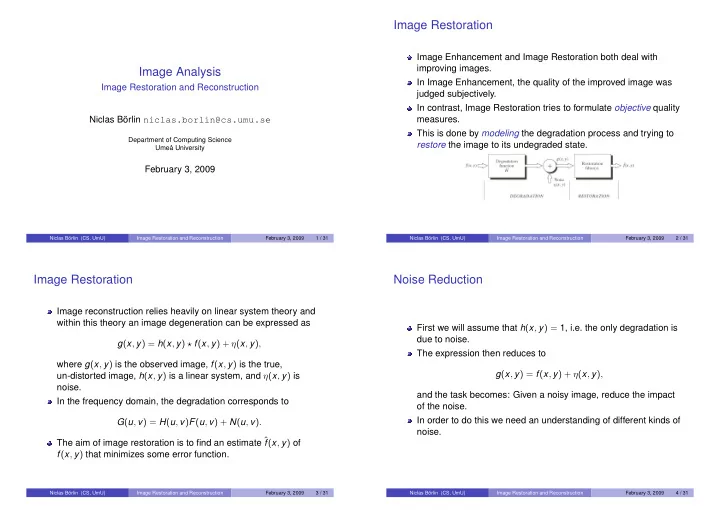
Image Enhancement and Image Restoration both deal with improving images. In Image Enhancement, the quality of the improved image was judged subjectively. In contrast, Image Restoration tries to formulate objective quality measures. This is done by modeling the degradation process and trying to restore the image to its undegraded state.

Niclas Börlin (CS, UmU) Image Restoration and Reconstruction February 3, 2009 2 / 31

Image Restoration

Image reconstruction relies heavily on linear system theory and within this theory an image degeneration can be expressed as g(x, y) = h(x, y) ⋆ f(x, y) + η(x, y), where g(x, y) is the observed image, f(x, y) is the true, un-distorted image, h(x, y) is a linear system, and η(x, y) is noise. In the frequency domain, the degradation corresponds to G(u, v) = H(u, v)F(u, v) + N(u, v). The aim of image restoration is to find an estimate ˆ f(x, y) of f(x, y) that minimizes some error function.

Niclas Börlin (CS, UmU) Image Restoration and Reconstruction February 3, 2009 3 / 31

Noise Reduction

First we will assume that h(x, y) = 1, i.e. the only degradation is due to noise. The expression then reduces to g(x, y) = f(x, y) + η(x, y), and the task becomes: Given a noisy image, reduce the impact

• f the noise.

In order to do this we need an understanding of different kinds of noise.

Niclas Börlin (CS, UmU) Image Restoration and Reconstruction February 3, 2009 4 / 31

Noise Reduction

Noise is here a stochastic component that is added to an intensity value. We will talk about two different kinds of noise: Position-independent noise and periodic noise. For position-independent noise we assume that the properties are global for the image, i.e. there is no spatial correlation tied to the properties of the noise. The values of a stochastic variable are generally described by its probability density function.

Niclas Börlin (CS, UmU) Image Restoration and Reconstruction February 3, 2009 5 / 31

Gaussian noise

The most common density function to use is the Gaussian (normal) distribution defined by p(z) = 1 √ 2πσ e−(z−¯

z)2/2σ2,

where ¯ z is the mean value (average) of the distribution, σ2 is the variance of the distribution. About 70% of the probability mass lies in the interval ¯ z ± σ and about 95% of the mass is in the interval ¯ z ± 2σ. The normal distribution is symmetric about its mean and is thus not optimal to model non-symmetric noise.

Niclas Börlin (CS, UmU) Image Restoration and Reconstruction February 3, 2009 6 / 31

Rayleigh noise (?)

The Rayleigh pdf is defined as p(z) = 2

b(z − a)e−(z−a)2/b

for z ≥ a

• therwise .

For this distribution, ¯ z = a +

• πb/4 and σ2 = b(4 − π)/4.

The Rayleigh is an example

• f an unsymmetric pdf.

Niclas Börlin (CS, UmU) Image Restoration and Reconstruction February 3, 2009 7 / 31

Erlang (gamma) noise

The Erlang (gamma) pdf is defined as p(z) =

• abzb−1

(b−1)! e−az

for z ≥ 0

• therwise ,

with ¯ z = a/b and σ2 = b/a2.

Niclas Börlin (CS, UmU) Image Restoration and Reconstruction February 3, 2009 8 / 31

Exponential noise

The Exponential pdf is p(z) = ae−az for z ≥ 0 for z < 0 and has ¯ z = 1/a and σ2 = 1/a2.

Niclas Börlin (CS, UmU) Image Restoration and Reconstruction February 3, 2009 9 / 31

Uniform noise

The density function for a uniform distribution is given by p(z) =

• 1

b−a

for a ≤ z ≥ b

• therwise

and has ¯ z = (a + b)/2 and σ2 = (b − a)2/12.

Niclas Börlin (CS, UmU) Image Restoration and Reconstruction February 3, 2009 10 / 31

Salt and pepper noise

And finally the pdf for salt and pepper noise p(z) =    Pa for z = a Pb for z = b

• therwise

with ¯ z = aPa + bPb and σ2 = Pbb2 + Paa2 − ¯ z.

Niclas Börlin (CS, UmU) Image Restoration and Reconstruction February 3, 2009 11 / 31

Noise test images

Niclas Börlin (CS, UmU) Image Restoration and Reconstruction February 3, 2009 12 / 31

Periodic noise

The noise can also be periodic. Any pure sinusoidal structure will appear as a pair of peaks in the spektra on opposite sides of the zero frequency in the spectra of the image. The distance from the zero frequency corresponds to the frequency of the structure.

Niclas Börlin (CS, UmU) Image Restoration and Reconstruction February 3, 2009 13 / 31

Periodic noise

Noisy image Fourier spectra, log scale linear scale linear scale, no DC

Niclas Börlin (CS, UmU) Image Restoration and Reconstruction February 3, 2009 14 / 31

Determining the noise type

If the noise is periodic, we will see it in the image and/or in the Fourier spectrum. Otherwise, we need to approximately determine the pdf to be able to choose what filter to use. In some cases we might know something about the source(s) of the noise.

◮ Gaussian-type noise often occur due to electronic circuit noise

and sensor noise due to poor illumination.

◮ Rayleigh noise may occur in application dealing with range

images.

◮ Exponential and Gamma distributions are useful for modeling

noise in relation to laser imaging.

◮ Impulse noise (salt and pepper) occur where we have quick

transients (faulty switches, strong radiation).

◮ Uniform noise is sometimes used for theoretical studies. Niclas Börlin (CS, UmU) Image Restoration and Reconstruction February 3, 2009 15 / 31

Determining the noise type

We may also study the histogram of a part of the image that should be homogenous. If we calculate the mean and variance of the noise, we may be able to estimate the parameters for the density functions.

Niclas Börlin (CS, UmU) Image Restoration and Reconstruction February 3, 2009 16 / 31

Spatial filtering for noise reduction, mean filters

Unless the noise is periodic it is hard to do something in the frequency domain. This leaves us with spatial filtering. The simplest approach to noise reduction is to smooth the image by using an average filter of size m × n ˆ f(x, y) = 1 mn

• (s,t)∈Sxy

g(s, t). This is also known as the Arithmetic mean. This will be quite effective to any noise with zero mean. The disadvantage is that sharp edges will be blurred.

Niclas Börlin (CS, UmU) Image Restoration and Reconstruction February 3, 2009 17 / 31

The geometric mean filter

There are other definitions of the mean that suite our purpose better than the arithmetic mean. The geometric mean is defined as ˆ f(x, y) =  

• (s,t)∈Sxy

g(s, t)  

1 mn

Smooths in the same way as the arithmetic mean, but tend to lose less details in the image.

Niclas Börlin (CS, UmU) Image Restoration and Reconstruction February 3, 2009 18 / 31

Harmonic means

The harmonic mean is defined as ˆ f(x, y) = 1 mn−1

• (s,t)∈Sxy

g(s, t)−1 = mn

• (s,t)∈Sxy

1 g(s,t)

. Works well for Gaussian and salt noise, fails for pepper noise. The contraharmonic mean is defined as ˆ f(x, y) =

• (s,t)∈Sxy g(s, t)Q+1
• (s,t)∈Sxy g(s, t)Q

Note that the contraharmonic mean reduces to the arithmetic mean for Q = 0 and the harmonic mean if Q = −1 With positive values of Q it is well suited for pepper noise and with negative values it is well suited for salt noise

Niclas Börlin (CS, UmU) Image Restoration and Reconstruction February 3, 2009 19 / 31

Order-statistic filters

Recall that the response of a order statistic filters are based on sorting the intensity values in a neighborhood Sxy. The simplest versions are the min, median and max filters. There are also hybrid filters that combine sorting with averaging. A midpoint filter is defined as ˆ f(x, y) = 1 2

• max

(s,t)∈Sxy

(g(s, t)) + min

(s,t)∈Sxy

(g(s, t)))

• This filter works best for Gaussian or uniform noise.

Niclas Börlin (CS, UmU) Image Restoration and Reconstruction February 3, 2009 20 / 31

Alpha-trimmed filters

The alpha-trimmed filter removes the d/2 lowest and d/2 highest values of the mn values in the neighborhood Sxy. The average value of the remaining mn − d values are used to represent the neighborhood. For d = 0 this filter reduces to an arithmetic mean filter. For d = (mn − 1)/2 the filter reduces to a median filter. The filter is suitable for noise with combined properties, such as Gaussian mixed with salt and pepper noise.

Niclas Börlin (CS, UmU) Image Restoration and Reconstruction February 3, 2009 21 / 31

Adaptive filters

By incorporating local statistics and other methods it is possible to construct adaptive filters. Adaptive filters are capable of performing superior noise reduction compared to non-adaptive filters.

Niclas Börlin (CS, UmU) Image Restoration and Reconstruction February 3, 2009 22 / 31

Adaptive, local noise reduction filters

It is assumed that we know the following

◮ the observed pixel g(x, y), ◮ the noise variance σ2

η,

◮ the local mean mL of pixels in Sxy, and ◮ the local variance σ2

L of pixels in Sxy.

We want the filter to have the following properties (for each (x, y))

◮ If σ2

η = 0 do nothing.

◮ If σ2

L is high in comparison to σ2 η return close to g(x, y).

◮ If σ2

η ≈ σ2 L return mL.

An implementation that does approximately this is ˆ f(x, y) = g(x, y) − σ2

η

σ2

L

(g(x, y) − mL)

Niclas Börlin (CS, UmU) Image Restoration and Reconstruction February 3, 2009 23 / 31

An adaptive median filter

Define

◮ zmin = min(Sxy). ◮ zmax = max(Sxy). ◮ zmed = median(Sxy). ◮ zxy = g(x, y). ◮ Smax largest allowed neighborhood size of Sxy.

Algorithm A1 If zmed = zmax, zmin goto B1 A2 Increase if size < Smax goto A1 A3 Return zmed B1 If zxy = zmin, zmax return zxy B2 Return zmed

Niclas Börlin (CS, UmU) Image Restoration and Reconstruction February 3, 2009 24 / 31

Frequency domain filtering

In order to reduce the effect of periodic noise we have to reduce the impact of specific frequencies of frequency bands. This is done by using either a bandreject filter or a notch filter. A bandreject filter reduce the energy of specific frequency bands. A notch filter reduce the energy of specific frequencies.

Niclas Börlin (CS, UmU) Image Restoration and Reconstruction February 3, 2009 25 / 31

Bandreject filters

A Gaussian bandreject filter is given by H(u, v) = 1 − e

− »

D2(u,v)−D2 DW

–2

, where D0 is the center rejection frequency and DW is the width

• f the filter.

|G(U, V)| in yellow, H(U, V) in blue. H(u, v)

Niclas Börlin (CS, UmU) Image Restoration and Reconstruction February 3, 2009 26 / 31

Bandreject noise reduction

|G(u, v)|H(u, v), lin scale |G(u, v)|H(u, v), log scale reconstructed image |G(u, v)|(1 − H(u, v)), lin scale |G(u, v)|(1 − H(u, v)), log scale removed noise

Niclas Börlin (CS, UmU) Image Restoration and Reconstruction February 3, 2009 27 / 31

Notch filters

When using notch filters we need to know the distance to a frequency (u0, v0) and since the spectra is symmetric we have

D1(u, v) =

• (u − u0)2 + (v − v0)2 and D2(u, v) =
• (u + u0)2 + (v + v0)2.

A Gaussian notch filter is defined as H(u, v) = 1 − e

− 1

2

»

D1(u,v)D2(u,v) D2

–

.

|G(U, V)| in yellow, H(U, V) in blue. H(u, v)

Niclas Börlin (CS, UmU) Image Restoration and Reconstruction February 3, 2009 28 / 31

Bandreject noise reduction

|G(u, v)|H(u, v), lin scale |G(u, v)|H(u, v), log scale reconstructed image |G(u, v)|(1 − H(u, v)), lin scale |G(u, v)|(1 − H(u, v)), log scale removed noise

Niclas Börlin (CS, UmU) Image Restoration and Reconstruction February 3, 2009 29 / 31

Weighted (modulated) notch filtering

In ideal cases the spikes of the periodic pattern are very well defined and are easily detected and removed. In more realistic cases the spikes can have a broad base that also carries information about the noise and should be removed. In these cases a simple notch filter will not perform very well. By using an estimate of the frequencies HNP(u, v) that make up the periodic pattern we can create the spectra of the noise as N(u, v) = HNP(u, v)G(u, v) Consequently we have η(x, y) = F−1{HNP(u, v)G(u, v)} The idea is to reconstruct f(x, y) by using ˆ f(x, y) = g(x, y) − w(x, y)η(x, y) where w(x, y) are local weights.

Niclas Börlin (CS, UmU) Image Restoration and Reconstruction February 3, 2009 30 / 31

Weighted (modulated) notch filtering

Normally we construct the weights w(x, y) so that the reconstructed image meets some criteria. A suitable criteria is to ensure that the local variance of ˆ f(x, y) is kept minimal. We denote the local variance in a neighborhood as σ2

L and the

local average of a function as g(x, y). By assuming that w(x, y) is constant within an m × n neighborhood it can be shown that w(x, y) = g(x, y)η(x, y) − g(x, y)η(x, y η2(x, y) − η2(x, y solves δσ2(x, y) δw(x, y) = 0.

Niclas Börlin (CS, UmU) Image Restoration and Reconstruction February 3, 2009 31 / 31