Introduction Decision Tree for PlayTennis (Mitchell) CSCE CSCE - - PDF document

SLIDE 1

CSCE 478/878 Lecture 3: Learning Decision Trees Stephen Scott Introduction Outline Tree Representation Learning Trees Inductive Bias Overfitting Tree Pruning

Introduction

Decision trees form a simple, easily-interpretable, hypothesis Interpretability useful in independent validation and explanation Quick to train Quick to evaluate new instances Effective “off-the-shelf” learning method Can be combined with boosting, including using “stumps”

2 / 26 CSCE 478/878 Lecture 3: Learning Decision Trees Stephen Scott Introduction Outline Tree Representation Learning Trees Inductive Bias Overfitting Tree Pruning

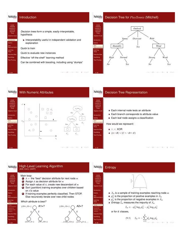
Decision Tree for PlayTennis (Mitchell)

Outlook Overcast Humidity Normal High No Yes Wind Strong Weak No Yes Yes Rain Sunny

4 / 26 CSCE 478/878 Lecture 3: Learning Decision Trees Stephen Scott Introduction Outline Tree Representation Learning Trees Inductive Bias Overfitting Tree Pruning

With Numeric Attributes

x

2

x

1

w

10

w

20

x

1

>w

10

x

2

>w

20

Yes No No Yes C

1

C

1

C

1

C

2

C

2

5 / 26 CSCE 478/878 Lecture 3: Learning Decision Trees Stephen Scott Introduction Outline Tree Representation Learning Trees Inductive Bias Overfitting Tree Pruning

Decision Tree Representation

Each internal node tests an attribute Each branch corresponds to attribute value Each leaf node assigns a classification How would we represent: ∧, ∨, XOR (A ∧ B) ∨ (C ∧ ¬D ∧ E)

6 / 26 CSCE 478/878 Lecture 3: Learning Decision Trees Stephen Scott Introduction Outline Tree Representation Learning Trees

High-Level Algorithm Entropy Learning Algorithm Example Run Regression Trees Variations

Inductive Bias Overfitting Tree Pruning

High-Level Learning Algorithm

(ID3, C4.5, CART)

Main loop:

1

A ← the “best” decision attribute for next node m

2

Assign A as decision attribute for m

3

For each value of A, create new descendant of m

4

Sort (partition) training examples over children based

• n A’s value

5

If training examples perfectly classified, Then STOP , Else recursively iterate over new child nodes Which attribute is best?

A1=? A2=? f t f t

[29+,35-] [29+,35-] [21+,5-] [8+,30-] [18+,33-] [11+,2-]

7 / 26 CSCE 478/878 Lecture 3: Learning Decision Trees Stephen Scott Introduction Outline Tree Representation Learning Trees

High-Level Algorithm Entropy Learning Algorithm Example Run Regression Trees Variations

Inductive Bias Overfitting Tree Pruning

Entropy

Entropy(S) 1.0 0.5 0.0 0.5 1.0 p+

Xm is a sample of training examples reaching node m p

m is the proportion of positive examples in Xm

p

m is the proportion of negative examples in Xm

Entropy Im measures the impurity of Xm Im ≡ −p

m log2 p m − p m log2 p m

• r for K classes,

(9.3) Im ≡ −

K

X

i=1

pi

m log2 pi m

8 / 26

SLIDE 2

CSCE 478/878 Lecture 3: Learning Decision Trees Stephen Scott Introduction Outline Tree Representation Learning Trees

High-Level Algorithm Entropy Learning Algorithm Example Run Regression Trees Variations

Inductive Bias Overfitting Tree Pruning

Total Impurity

Now can look for an attribute A, when used to partition Xm by value, produces the most pure (lowest-entropy) subsets

Weight each subset by relative size E.g., size-3 subsets should carry less influence than size-300 ones

Let Nm = |Xm| = number of instances reaching node m Let Nmj = number of these instances with value j ∈ {1, . . . , n} for attribute A Let Ni

mj = number of these instances with label

i ∈ {1, . . . , K} Let pi

mj = Ni mj/Nmj

Then the total impurity is (9.8) I0

m(A) ≡ − n

X

j=1

Nmj Nm

K

X

i=1

pi

mj log2 pi mj

9 / 26 CSCE 478/878 Lecture 3: Learning Decision Trees Stephen Scott Introduction Outline Tree Representation Learning Trees

High-Level Algorithm Entropy Learning Algorithm Example Run Regression Trees Variations

Inductive Bias Overfitting Tree Pruning

Learning Algorithm

10 / 26 CSCE 478/878 Lecture 3: Learning Decision Trees Stephen Scott Introduction Outline Tree Representation Learning Trees

High-Level Algorithm Entropy Learning Algorithm Example Run Regression Trees Variations

Inductive Bias Overfitting Tree Pruning

Example Run

Training Examples Day Outlook Temperature Humidity Wind PlayTennis D1 Sunny Hot High Weak No D2 Sunny Hot High Strong No D3 Overcast Hot High Weak Yes D4 Rain Mild High Weak Yes D5 Rain Cool Normal Weak Yes D6 Rain Cool Normal Strong No D7 Overcast Cool Normal Strong Yes D8 Sunny Mild High Weak No D9 Sunny Cool Normal Weak Yes D10 Rain Mild Normal Weak Yes D11 Sunny Mild Normal Strong Yes D12 Overcast Mild High Strong Yes D13 Overcast Hot Normal Weak Yes D14 Rain Mild High Strong No

11 / 26 CSCE 478/878 Lecture 3: Learning Decision Trees Stephen Scott Introduction Outline Tree Representation Learning Trees

High-Level Algorithm Entropy Learning Algorithm Example Run Regression Trees Variations

Inductive Bias Overfitting Tree Pruning

Example Run

Selecting the First Attribute

Comparing Humidity to Wind:

High Normal Humidity [3+,4-] [6+,1-] Wind Weak Strong [6+,2-] [3+,3-] =0.940 E =0.940 E =0.811 E =0.592 E =0.985 E =1.00 E [9+,5-] S: [9+,5-] S:

I0

m(Humidity) = (7/14)0.985 + (7/14)0.592 = 0.789

I0

m(Wind) = (8/14)0.811 + (6/14)1.000 = 0.892

I0

m(Outlook) = (5/14)0.971 + (4/14)0.0 + (5/14)0.971 = 0.694

I0

m(Temp) = (4/14)1.000 + (6/14)0.918 + (4/14)0.811 = 0.911

12 / 26 CSCE 478/878 Lecture 3: Learning Decision Trees Stephen Scott Introduction Outline Tree Representation Learning Trees

High-Level Algorithm Entropy Learning Algorithm Example Run Regression Trees Variations

Inductive Bias Overfitting Tree Pruning

Example Run

Selecting the Next Attribute

Outlook Sunny Overcast Rain [9+,5] {D1,D2,D8,D9,D11} {D3,D7,D12,D13} {D4,D5,D6,D10,D14} [2+,3] [4+,0] [3+,2] Yes {D1, D2, ..., D14}

? ? Which attribute should be tested here?

• Xm = {D1, D2, D8, D9, D11}

I0

m(Humidity) = (3/5)0.0 + (2/14)0.0 = 0.0

I0

m(Wind) = (2/5)1.0 + (3/5)0.918 = 0.951

I0

m(Temp) = (2/5)0.0 + (2/5)1.0 + (1/5)0.0 = 0.400

13 / 26 CSCE 478/878 Lecture 3: Learning Decision Trees Stephen Scott Introduction Outline Tree Representation Learning Trees

High-Level Algorithm Entropy Learning Algorithm Example Run Regression Trees Variations

Inductive Bias Overfitting Tree Pruning

Regression Trees

A regression tree is similar to a decision tree, but with real-valued labels at the leaves To measure impurity at a node m, replace entropy with variance of labels: Em ≡ 1 Nm X

(xt,rt)2Xm

(rt − gm)2 , where gm is the mean (or median) label in Xm

14 / 26

SLIDE 3

CSCE 478/878 Lecture 3: Learning Decision Trees Stephen Scott Introduction Outline Tree Representation Learning Trees

High-Level Algorithm Entropy Learning Algorithm Example Run Regression Trees Variations

Inductive Bias Overfitting Tree Pruning

Regression Trees (cont’d)

Now can adapt Eq. (9.8) from classification to regression: E0

m(A) ≡ n

X

j=1

Nmj Nm @ 1 Nmj X

(xt,rt)2Xmj

(rt − gmj)2 1 A (9.14) = 1 Nm

n

X

j=1

X

(xt,rt)2Xmj

(rt − gmj)2 , where j iterates over the values of attribute A When variance of a subset is sufficiently low, insert leaf with mean or median label as constant value

15 / 26 CSCE 478/878 Lecture 3: Learning Decision Trees Stephen Scott Introduction Outline Tree Representation Learning Trees

High-Level Algorithm Entropy Learning Algorithm Example Run Regression Trees Variations

Inductive Bias Overfitting Tree Pruning

Continuous-Valued Attributes

Use threshold to map continuous to boolean, e.g. (Temperature > 72.3) ∈ {t, f} Temperature: 40 48 60 72 80 90 PlayTennis: No No Yes Yes Yes No Can show that threshold minimizing impurity must lie between two adjacent attribute values in X such that label changed, so try all such values, e.g., (48 + 60)/2 = 54 and (80 + 90)/2 = 85 Now (dynamically) replace continuous attribute with boolean attributes Temperature>54 and Temperature>85 and run algorithm normally Other options: Split into multiple intervals rather than two; use thresholded linear combinations of continuous attributes (Sec 9.6)

16 / 26 CSCE 478/878 Lecture 3: Learning Decision Trees Stephen Scott Introduction Outline Tree Representation Learning Trees

High-Level Algorithm Entropy Learning Algorithm Example Run Regression Trees Variations

Inductive Bias Overfitting Tree Pruning

Attributes with Many Values

Problem: If attribute A has many values, it might artificially minimize I0

m(A)

E.g., if Date is attribute, I0

m(A) will be low because

several very small subsets will be created One approach: penalize A with a measure of split information, which measures how broadly and uniformly attribute A splits data: S(A) ≡ −

n

X

j=1

Nmj Nm log2 Nmj Nm ∈ [0, log2 n]

17 / 26 CSCE 478/878 Lecture 3: Learning Decision Trees Stephen Scott Introduction Outline Tree Representation Learning Trees

High-Level Algorithm Entropy Learning Algorithm Example Run Regression Trees Variations

Inductive Bias Overfitting Tree Pruning

Unknown Attribute Values

What if a training example is missing a value of A? Use it anyway (sift it through tree) If node m tests A, assign most common value of A among other training examples sifted to m Assign most common value of A among other examples with same target value (either overall or at m) Assign probability pj to each possible value vj of A

Assign fraction pj of example to each descendant in tree

Classify new examples in same fashion

18 / 26 CSCE 478/878 Lecture 3: Learning Decision Trees Stephen Scott Introduction Outline Tree Representation Learning Trees Inductive Bias Overfitting Tree Pruning

Inductive Bias of Learning Algorithm

Hypothesis space H is complete, in that any function can be represented Thus inductive bias does not come from restricting H, but from preferring some trees over others

Tends to prefer shorter trees Computationally intractable to find a guaranteed shortest tree, so heuristically apply greedy approach to locally minimize impurity

19 / 26 CSCE 478/878 Lecture 3: Learning Decision Trees Stephen Scott Introduction Outline Tree Representation Learning Trees Inductive Bias Overfitting Tree Pruning

Overfitting

Consider adding noisy training example #15: Sunny, Hot, Normal, Strong, PlayTennis = No What effect on earlier tree?

Outlook Overcast Humidity Normal High No Yes Wind Strong Weak No Yes Yes Rain Sunny

Expect old tree to generalize better since new one fits noisy example

20 / 26

SLIDE 4

CSCE 478/878 Lecture 3: Learning Decision Trees Stephen Scott Introduction Outline Tree Representation Learning Trees Inductive Bias Overfitting Tree Pruning

Overfitting (cont’d)

Consider error of hypothesis h over

training data (empirical error): errortrain(h) entire distribution D of data (generalization error): errorD(h)

Hypothesis h ∈ H overfits training data if there is an alternative hypothesis h0 ∈ H such that errortrain(h) < errortrain(h0) and errorD(h) > errorD(h0)

21 / 26 CSCE 478/878 Lecture 3: Learning Decision Trees Stephen Scott Introduction Outline Tree Representation Learning Trees Inductive Bias Overfitting Tree Pruning

Overfitting (cont’d)

0.5 0.55 0.6 0.65 0.7 0.75 0.8 0.85 0.9 10 20 30 40 50 60 70 80 90 100 Accuracy Size of tree (number of nodes) On training data On test data

22 / 26 CSCE 478/878 Lecture 3: Learning Decision Trees Stephen Scott Introduction Outline Tree Representation Learning Trees Inductive Bias Overfitting Tree Pruning

Rule Postpruning

Pruning to Avoid Overfitting

To prevent trees from growing too much and overfitting the data, we can prune them

In spirit of Occam’s Razor, minimum description length

In prepruning, we allow skipping a recursive call on set Xm and instead insert a leaf, even if Xm is not pure

Can do this when entropy (or variance) is below a threshold (θI in pseudocode) Can do this when |Xm| is below a threshold, e.g., 5

In postpruning, we grow the tree until it has zero error

• n training set and then prune it back afterwards

First, set aside a pruning set not used in initial training Then repeat until pruning is harmful:

1

Evaluate impact on validation set of pruning each possible node (plus those below it)

2

Greedily remove the one that most improves validation set accuracy

23 / 26 CSCE 478/878 Lecture 3: Learning Decision Trees Stephen Scott Introduction Outline Tree Representation Learning Trees Inductive Bias Overfitting Tree Pruning

Rule Postpruning

Pruning Example

0.5 0.55 0.6 0.65 0.7 0.75 0.8 0.85 0.9 10 20 30 40 50 60 70 80 90 100 Accuracy Size of tree (number of nodes) On training data On test data On test data (during pruning)

24 / 26 CSCE 478/878 Lecture 3: Learning Decision Trees Stephen Scott Introduction Outline Tree Representation Learning Trees Inductive Bias Overfitting Tree Pruning

Rule Postpruning

Rule Postpruning

Convert tree to equivalent set of rules Prune each rule independently of others by removing selected preconditions (the ones that improve accuracy the most) Sort final rules into desired sequence for use Perhaps most frequently used method (e.g. C4.5)

25 / 26 CSCE 478/878 Lecture 3: Learning Decision Trees Stephen Scott Introduction Outline Tree Representation Learning Trees Inductive Bias Overfitting Tree Pruning

Rule Postpruning

Converting A Tree to Rules

Outlook Overcast Humidity Normal High No Yes Wind Strong Weak No Yes Yes Rain Sunny

IF (Outlook = Sunny) ∧ (Humidity = High) THEN PlayTennis = No IF (Outlook = Sunny) ∧ (Humidity = Normal) THEN PlayTennis = Yes . . .

26 / 26