Introduction to Recurrent Neural Networks Jakob Verbeek Modeling - - PowerPoint PPT Presentation

introduction to recurrent neural networks
SMART_READER_LITE
LIVE PREVIEW

Introduction to Recurrent Neural Networks Jakob Verbeek Modeling - - PowerPoint PPT Presentation

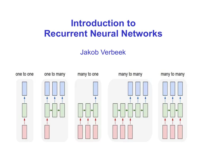
Introduction to Recurrent Neural Networks Jakob Verbeek Modeling sequential data with Recurrent Neural Networks Compact schematic drawing of standard multi-layer perceptron (MLP) output hidden input Modeling sequential data So far we


slide-1
SLIDE 1

Introduction to Recurrent Neural Networks

Jakob Verbeek

slide-2
SLIDE 2

Modeling sequential data with Recurrent Neural Networks

Compact schematic drawing of standard multi-layer perceptron (MLP)

input

  • utput

hidden

slide-3
SLIDE 3

Modeling sequential data

So far we considered “one-to-one” prediction tasks

Classification: one image to one class label, which digit is displayed 0...9

Regression: one image to one scalar, how old is this person?

Many prediction problems have a sequential nature to them

Either in input, in output, or both

Both may vary in length from one example to another

slide-4
SLIDE 4

Modeling sequential data

One-to-many prediction

Image captioning

Input: an image

Output: natural language description, variable length sequence of words

slide-5
SLIDE 5

Modeling sequential data

Text classification

Input: a sentence

Output: user rating

slide-6
SLIDE 6

Modeling sequential data

Machine translation of text from one language to another

Sequences of different length on input and output

slide-7
SLIDE 7

Modeling sequential data

Part of speech tagging

For each word in sentence predict PoS label (verb, noun, adjective, etc.)

Temporal segmentation of video

Predict action label for every video frame

Temporal segmentation of audio

Predict phoneme labels over time

slide-8
SLIDE 8

Modeling sequential data

Possible to use a k-order autoregressive model over output sequences

Limits memory to only k time steps in the past

Not applicable when input sequence is not aligned with output sequence

Many-to-one tasks, unaligned many-to-many

slide-9
SLIDE 9

Recurrent neural networks

Recurrent computation of hidden units from one time step to the next

Hidden state accumulates information on entire sequence, since the field

  • f view spans entire sequence processed so far

Time-invariant function makes it applicable to arbitrarily long sequences

Similar ideas used in

Hidden Markov models for arbitrarily long sequences

Parameter sharing across space in convolutional neural networks

But has limited field of view: parallel instead of sequential processing

slide-10
SLIDE 10

Recurrent neural networks

Basic example for many-to-many prediction

Hidden state linear function of current input and previous hidden state, followed by point-wise non-linearity

Output is linear function of current hidden state, followed by point-wise non-linearity zt=ϕ( A xt+B zt−1)

yt=ψ(C zt) xt yt zt

slide-11
SLIDE 11

Recurrent neural network diagrams

Two graphical representations are used “Unfolded” flow diagram Recurrent flow diagram

Unfolded representation shows that we still have an acyclic directed graph

Size of the graph (horizontally) is variable, given by sequence length

Weights are shared across horizontal replications

Gradient computation via back-propagation as before

Referred to as “back-propagation through time” (Pearlmutter, 1989) xt yt zt xt yt zt A B C zt=ϕ (A xt+B zt−1) yt=ψ(C zt)

slide-12
SLIDE 12

Recurrent neural network diagrams

Deterministic feed-forward network from inputs to outputs

Predictive model over output sequence is obtained by defining a distribution

  • ver outputs given y

For example: probability of a word given via softmax of word score

Training loss: sum of losses over output variables

Independent prediction of elements in output given input sequence p(wt=k∣x1:t)= exp ytk

∑v=1

V

exp ytv xt yt zt zt=ϕ( A xt+B zt−1) yt=ψ(C zt) wt L=−∑t=1

T

ln p(wt∣x1:t)

slide-13
SLIDE 13

More topologies: “deep” recurrent networks

Instead of a recurrence across a single hidden layer, consider a recurrence across a multi-layer architecture x

t

h

t

z

t

y

t

x

t

h

t

z

t

y

t

x

t

h

t

z

t

y

t

x

t

h

t

z

t

y

t

slide-14
SLIDE 14

More topologies: multi-dimensional recurrent networks

Instead of a recurrence across a single (time) axis, consider a recurrence across a multi-dimensional grid

For example: axis aligned directed edges

Each node receives input from predecessors, one for each dimension x

3,1

x

3,3

x

3,2

x

2,1

x

2,3

x

2,2

x

1,1

x

1,3

x

1,2

x

3,1

x

3,3

x

3,2

x

2,1

x

2,3

x

2,2

x

1,1

x

1,3

x

1,2

slide-15
SLIDE 15

More topologies: bidirectional recurrent neural networks

Standard RNN only uses left-context for many-to-many prediction

Use two separate recurrences, one in each direction

Aggregate output from both directions for prediction at each time step

Only possible on a given input sequence of arbitrary length

Not on output sequence, since it needs to be predicted/generated

slide-16
SLIDE 16

More topologies: output feedback loops

So far the element in the output sequence at time t was independently drawn given the state at time t

State at time t depends on the entire input sequence up to time t

No dependence on the output sequence produced so far

Problematic when there are strong regularities in output, eg character or words sequences in natural language xt yt zt p(w1:T∣x1:T)=∏t=1

T

p(wt∣x1:t)

slide-17
SLIDE 17

More topologies: output feedback loops

To introduce dependence on output sequence, we add a feedback loop from the output to the hidden state

Without output-feedback, the state evolution is a deterministic non-linear dynamical system

With output feedback, the state evolution becomes a stochastic non-linear dynamical system

Caused by the stochastic output, which flows back into the state update xt yt zt p( y1:T∣x1:T)=∏t=1

T

p( yt∣x1:t, y1:t−1)

slide-18
SLIDE 18

How do we generate data from an RNN ?

xt yt zt

RNN gives a distribution over output sequences

Sampling: sequentially sample one element at a time

Compute state from current input and previous state and output

Compute distribution on current output symbol

Sample output symbol

Compute maximum likelihood sequence?

Not feasible with feedback since output symbol impacts state

Marginal distribution on n-th symbol

Not feasible: marginalize over exponential nr. of sequences

Marginal probability of a symbol appearing anywhere in seq.

Not feasible: average over all marginals

slide-19
SLIDE 19

Approximate maximum likelihood sequences

Exhaustive maximum likelihood search exponential in sequence length

Use Beam Search, computational cost linear in

Beam size K, vocabulary size V, (maximum) sequence length T

ϵ a a ϵ a b ϵ a b ϵ a b ϵ a b ϵ a b ϵ a b ϵ a b ϵ a b λ ϵ a b T = 3 T = 2 T = 1

current hypotheses proposed extensions current hypotheses proposed extensions current hypotheses proposed extensions empty string

slide-20
SLIDE 20

Ensembles of networks to improve prediction

Averaging predictions of several networks can improve results

Trained from different initialization and using different mini-batches

Possibly including networks with different architectures, but not per se

For CNNs see eg [Krizhevsky & Hinton, 2012] [Simomyan & Zisserman, 2014]

For RNN sequence prediction

Train RNNs independently

“Run” RNNs in parallel for prediction, updating states with common seq.

Average distribution over next symbol

Sample or beam-search based on av. distribution

A B ? A B ?

slide-21
SLIDE 21

How to train an RNN without output feedback?

xt yt zt

Compute full state sequence given the input (deterministic given input)

Compute loss at each time step w.r.t. ground truth output sequence

Backpropagation (“through time”) to compute gradients w.r.t. loss

slide-22
SLIDE 22

How to train an RNN with output feedback?

xt yt zt

Compute state sequence given input and ground-truth output, deterministic due to known and fixed output

Loss at each time step wrt ground truth output seq, backprop through time

Note discrepancy between train and test

Train: predict next symbol from ground-truth sequence so far

Test: predict next symbol from generated sequence so far

Might deviate from observed ground-truth sequences

slide-23
SLIDE 23

Scheduled sampling for RNN training

Compensate discrepancy between train and test procedure by training from generated sequence [Bengio et al. NIPS, 2015]

Learn to recover from partially incorrect sequences

Directly training from sampled sequences does not work well in practice

At the start randomly initialized model generates random sequences

Instead, start by training from ground-truth sequence, and progressively increase probability to sample generated symbol in the sequence

slide-24
SLIDE 24

Scheduled sampling for RNN training

Evaluation image captioning

Image in, sentence out

Higher scores are better

Scheduled sampling improves baseline, also in ensemble case

Uniform Scheduled Sampling: sample uniform instead of using model

Already improves over baseline, but not as much as using model

Always sampling gives very poor results, as expected

slide-25
SLIDE 25

Limitations recurrent networks

Recurrent net can be unrolled as deep network with shared parameters

As deep as the number of time steps of the RNN

Very deep for very long sequences

Gradients of “deep” layers (far from input) computed via chainrule as product

  • f Jacobians between layers (time-steps)

Product of Jacobians tend to either “explode” to inf. or “vanish” to zero

Similar effect observed in non-recurrent networks

Approaches to address this issue

Non-recurrent case: add skip connections from earlier layers towards

  • utput: Residual networks, dense networks

Introduction of “gates” that shield a hidden unit from input and/or output for several layers, effectively shortening the depth for that unit

slide-26
SLIDE 26

Long short-term memory (LSTM) cells

LSTM consist of hidden state h and a “memory cell” c

Gates are used to modulate the state updates [Hochreiter & Schmidhuber, Neural Computation, 1997]

slide-27
SLIDE 27

Long short-term memory (LSTM) cells

Introduced by Hochreiter & Schmidhuber (Neural Computation, 1997)

LSTM defines a dynamical system on hidden state h and a “memory cell” c

Involves a number of additional processing elements

Cell update: can forget previous cell state, can ignore input

slide-28
SLIDE 28

Long short-term memory (LSTM) cells

Introduced by Hochreiter & Schmidhuber (Neural Computation, 1997)

LSTM defines a dynamical system on hidden state h and a “memory cell” c

Involves a number of additional processing elements

Forget gate f: “remember” or “forget” previous cell state c

slide-29
SLIDE 29

Long short-term memory (LSTM) cells

Introduced by Hochreiter & Schmidhuber (Neural Computation, 1997)

LSTM defines a dynamical system on hidden state h and a “memory cell” c

Involves a number of additional processing elements

Input gate i: controls flow of input to cell state

Input modulator , maps input and previous state to cell state update ~ C

slide-30
SLIDE 30

Long short-term memory (LSTM) cells

Introduced by Hochreiter & Schmidhuber (Neural Computation, 1997)

LSTM defines a dynamical system on hidden state h and a “memory cell” c

Involves a number of additional processing elements

Output gate o, controls flow of cell state to output

Output vector also passed to next time step of LSTM unit

slide-31
SLIDE 31

Gated Recurrent Unit (GRU) cells

GRU is simplified gated RNN as compared to LSTM [Cho et al., Empirical Methods in Natural Language Processing, 2014]

Two gates, single state signal

Forget gate: z

Read gate: r

slide-32
SLIDE 32

Examples of character-level LSTM language model

Training data: all Paul Graham essays, about 1 million characters

Random sample from the trained model: "The surprised in investors weren't going to raise money. I'm not the company with the time there are all interesting quickly, don't have to get off the same

  • programmers. There's a super-angel round fundraising, why do you can do. If

you have a different physical investment are become in people who reduced in a startup with the way to argument the acquirer could see them just that you're also the founders will part of users' affords that and an alternation to the idea. [2] Don't work at first member to see the way kids will seem in advance of a bad successful startup. And if you have to act the big company too."

Learns to spell words, as well as long range grammatical dependencies

[examples taken from Andrej Karpathy]

slide-33
SLIDE 33

Examples of character-level LSTM language model

Training data: all of Shakespeak (4.4 MB)

Random sample from the trained model:

PANDARUS: Alas, I think he shall be come approached and the day When little srain would be attain'd into being never fed, And who is but a chain and subjects of his death, I should not sleep. Second Senator: They are away this miseries, produced upon my soul, Breaking and strongly should be buried, when I perish The earth and thoughts of many states. DUKE VINCENTIO: Well, your wit is in the care of side and that. Second Lord: They would be ruled after this chamber, and my fair nues begun out of the fact, to be conveyed, Whose noble souls I'll have the heart of the wars. Clown: Come, sir, I will make did behold your worship. VIOLA: I'll drink it.

Specific style structure is also captured by the model

slide-34
SLIDE 34

Examples of character-level LSTM language model

Training data: linux source code (474 MB)

Very long range dependencies on bracket structure

/* * Increment the size file of the new incorrect UI_FILTER group information * of the size generatively. */ static int indicate_policy(void) { int error; if (fd == MARN_EPT) { /* * The kernel blank will coeld it to userspace. */ if (ss->segment < mem_total) unblock_graph_and_set_blocked(); else ret = 1; goto bail; } segaddr = in_SB(in.addr); selector = seg / 16; setup_works = true; for (i = 0; i < blocks; i++) { seq = buf[i++]; bpf = bd->bd.next + i * search; if (fd) { current = blocked; } } rw->name = "Getjbbregs"; bprm_self_clearl(&iv->version); regs->new = blocks[(BPF_STATS << info->historidac)] | PFMR_CLOBATHINC_SECONDS << 12; return segtable; }

slide-35
SLIDE 35

Case study: image captioning

Given image generate descriptive english sentence

slide-36
SLIDE 36

Image captioning with encoder-decoder system

Encoder: CNN takes image and maps it into a vector

For example, fully connected layer of VGG16 network

CNN pre-trained on ImageNet classification task (>1 million images)

slide-37
SLIDE 37

Image captioning with encoder-decoder system

Decoder: RNN takes CNN image vector to initialize RNN state

Typical configuration:

Single layer of 512 GRUs

Output feedback to ensure coherent sentence

slide-38
SLIDE 38

Image captioning with encoder-decoder system

Example output (Vinyals et al., CVPR 2015)

slide-39
SLIDE 39

Encoder-decoder machine translation

Translation of a sentence into another language

Input and output of different length

slide-40
SLIDE 40

Encoder-decoder machine translation

Read source sentence with encoder RNN (Sutskever et al., NIPS 2014)

Can use bidirectional RNN since input sequence is given

Generate target sentence with decoder RNN

Uses a different set of parameters

Uses output feedback to ensure output coherency

Meaning of source sentence encoded in the RNN state vector passed between encoder and decoder

For the captioning model, a CNN is used as an image encoder

encoder decoder

slide-41
SLIDE 41

Encoder-decoder machine translation

F i g u r e : K y u n g h y u n C h

Encoder learns a word embedding matrix E

Columns contain word vector embedding

si=Ewi

Decoder learns word embedding matrix G for

  • utput feedback

zi+1=ϕ(W zi+Gui)

Decoder learns word embedding matrix F for word probabilities via softmax normalization

pi=σ(F zi)

slide-42
SLIDE 42

Encoder-decoder machine translation

Trained from “aligned” corpus of matching source-target sentences

Encoder and decoder can be learned on multiple language pairs in parallel

(English to French) and (Dutch to French) use same decoder

(English to French) and (English to Dutch) use same encoder

Generalizes to translation between new language pairs for which no aligned training corpus was available

english french french english dutch english dutch english dutch english english dutch french french

slide-43
SLIDE 43

Encoder-decoder machine translation

PCA projection of LSTM encoder state after reading a sentence

Word order important for meaning, captured in encoder state vector

e n c

  • d

e r d e c

  • d

e r

slide-44
SLIDE 44

Attention mechanisms in RNNs

Encoder-decoder based models compress the entire input into a single vector

Difficult to store all details as the sentences grow longer

Sequential nature of RNN updates makes that start of sentence is less well encoded into the RNN state

Using bi-directional RNN helps, but not in the middle of the sentence...

slide-45
SLIDE 45

Attention mechanisms in RNNs

Let decoder attend to part of the input for each state update

Selectively: based on current state and input representation

Should work for input sequences of variable size

Sub-network takes state and input encoding, computes attention weights

Soft-max over candidate positions in the input

Feed weighted sum of inputs to the state update aij=σ(zi,h j) zi+1=ϕ(zi,ci,ui) ci=∑j=1

T

aijh j

[Bahdanau et al., ICLR’15]

slide-46
SLIDE 46

Attention mechanisms in RNNs

Example correspondences identified by attention mechanism

Trained from sentence-level supervision, no word correspondences

slide-47
SLIDE 47

Attention mechanisms in image captioning

Without attention image content encoded into vector output of CNN

Decoder cannot “look back” at image

Attention can be used to focus decoder model on parts of input [Xu et al, ICML’15]

slide-48
SLIDE 48

Attention mechanisms in image captioning

What are the image “parts” that we should be looking at?

[Pedersoli et al, ICCV’17]

Activation grid: the locations in a convolutional CNN layer

Object proposals: plausible object locations predicted by external method

Spatial transformer: regress deformation of default boxes at locations in activation grid

slide-49
SLIDE 49

Attention mechanisms in image captioning

Examples of generated sentences together with the attention regions

Region width proportional to attention weight [Pedersoli et al., ICCV’17]

slide-50
SLIDE 50

Further reading

“Pattern Recognition and Machine Learning” Chris Bishop. Springer, 2006.

“Supervised Sequence Labelling with Recurrent Neural Networks” Alex Graves, 2012 (free online)

“Deep Learning” Ian Goodfellow, Yoshua Bengio, Aaron Courville. MIT Press, in preparation. http://www.deeplearningbook.org/