Karl Theodor Wilhelm Weierstrass 31 October 1815 19 February 1897 - - PowerPoint PPT Presentation

karl theodor wilhelm weierstrass 31 october 1815 19
SMART_READER_LITE
LIVE PREVIEW

Karl Theodor Wilhelm Weierstrass 31 October 1815 19 February 1897 - - PowerPoint PPT Presentation

Happy Hallo WEIERSTRASS Did you know that Weierestrass was born on Halloween? Neither did we Dmitriy Bilyk will be speaking on Lacunary Fourier series: from Weierstrass to our days Monday, Oct 31 at 12:15pm in Vin 313 followed by Mesa


slide-1
SLIDE 1

Brought to you by the UMN AMS Student Chapter and

at 12:15pm in Vin 313 followed by Mesa Pizza in the first floor lounge

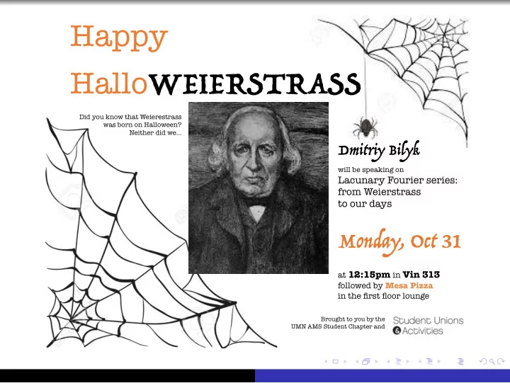
Did you know that Weierestrass was born on Halloween? Neither did we…

Happy HalloWEIERSTRASS

Monday, Oct 31

Dmitriy Bilyk

will be speaking on

Lacunary Fourier series: from Weierstrass to our days

slide-2
SLIDE 2

Karl Theodor Wilhelm Weierstrass 31 October 1815 – 19 February 1897

slide-3
SLIDE 3

Karl Theodor Wilhelm Weierstraß 31 October 1815 – 19 February 1897

slide-4
SLIDE 4

Karl Theodor Wilhelm Weierstraß 31 October 1815 – 19 February 1897

slide-5
SLIDE 5

Karl Theodor Wilhelm Weierstraß 31 October 1815 – 19 February 1897

born in Ostenfelde, Westphalia, Prussia.

slide-6
SLIDE 6

Karl Theodor Wilhelm Weierstraß 31 October 1815 – 19 February 1897

born in Ostenfelde, Westphalia, Prussia. sent to University of Bonn to prepare for a government position – dropped out.

slide-7
SLIDE 7

Karl Theodor Wilhelm Weierstraß 31 October 1815 – 19 February 1897

born in Ostenfelde, Westphalia, Prussia. sent to University of Bonn to prepare for a government position – dropped out. studied mathematics at the M¨ unster Academy.

slide-8
SLIDE 8

Karl Theodor Wilhelm Weierstraß 31 October 1815 – 19 February 1897

born in Ostenfelde, Westphalia, Prussia. sent to University of Bonn to prepare for a government position – dropped out. studied mathematics at the M¨ unster Academy. University of K¨

  • nigsberg gave him an honorary

doctor’s degree March 31, 1854.

slide-9
SLIDE 9

Karl Theodor Wilhelm Weierstraß 31 October 1815 – 19 February 1897

born in Ostenfelde, Westphalia, Prussia. sent to University of Bonn to prepare for a government position – dropped out. studied mathematics at the M¨ unster Academy. University of K¨

  • nigsberg gave him an honorary

doctor’s degree March 31, 1854. 1856 a chair at Gewerbeinstitut (now TU Berlin)

slide-10
SLIDE 10

Karl Theodor Wilhelm Weierstraß 31 October 1815 – 19 February 1897

born in Ostenfelde, Westphalia, Prussia. sent to University of Bonn to prepare for a government position – dropped out. studied mathematics at the M¨ unster Academy. University of K¨

  • nigsberg gave him an honorary

doctor’s degree March 31, 1854. 1856 a chair at Gewerbeinstitut (now TU Berlin) professor at Friedrich-Wilhelms-Universit¨ at Berlin (now Humboldt Universit¨ at)

slide-11
SLIDE 11

Karl Theodor Wilhelm Weierstraß 31 October 1815 – 19 February 1897

born in Ostenfelde, Westphalia, Prussia. sent to University of Bonn to prepare for a government position – dropped out. studied mathematics at the M¨ unster Academy. University of K¨

  • nigsberg gave him an honorary

doctor’s degree March 31, 1854. 1856 a chair at Gewerbeinstitut (now TU Berlin) professor at Friedrich-Wilhelms-Universit¨ at Berlin (now Humboldt Universit¨ at) died in Berlin of pneumonia

slide-12
SLIDE 12

Karl Theodor Wilhelm Weierstraß 31 October 1815 – 19 February 1897

born in Ostenfelde, Westphalia, Prussia. sent to University of Bonn to prepare for a government position – dropped out. studied mathematics at the M¨ unster Academy. University of K¨

  • nigsberg gave him an honorary

doctor’s degree March 31, 1854. 1856 a chair at Gewerbeinstitut (now TU Berlin) professor at Friedrich-Wilhelms-Universit¨ at Berlin (now Humboldt Universit¨ at) died in Berlin of pneumonia

  • ften cited as the father of modern analysis
slide-13
SLIDE 13

Doctoral students of Karl Weierstrass include

Georg Cantor Georg Frobenius Sofia Kovalevskaya Carl Runge Hans von Mangoldt Hermann Schwarz Magnus Gustaf (G¨

  • sta) Mittag-Leffler∗

Weierstrass’s doctoral advisor was Christoph Gudermann, a student of Carl Gauss.

slide-14
SLIDE 14

Things named after Weierstrass

Bolzano–Weierstrass theorem

slide-15
SLIDE 15

Things named after Weierstrass

Bolzano–Weierstrass theorem Weierstrass M-test

slide-16
SLIDE 16

Things named after Weierstrass

Bolzano–Weierstrass theorem Weierstrass M-test Weierstrass approximation theorem/Stone–Weierstrass theorem

slide-17
SLIDE 17

Things named after Weierstrass

Bolzano–Weierstrass theorem Weierstrass M-test Weierstrass approximation theorem/Stone–Weierstrass theorem Weierstrass–Casorati theorem

slide-18
SLIDE 18

Things named after Weierstrass

Bolzano–Weierstrass theorem Weierstrass M-test Weierstrass approximation theorem/Stone–Weierstrass theorem Weierstrass–Casorati theorem Hermite–Lindemann–Weierstrass theorem

slide-19
SLIDE 19

Things named after Weierstrass

Bolzano–Weierstrass theorem Weierstrass M-test Weierstrass approximation theorem/Stone–Weierstrass theorem Weierstrass–Casorati theorem Hermite–Lindemann–Weierstrass theorem Weierstrass elliptic functions (P-function)

slide-20
SLIDE 20

Things named after Weierstrass

Bolzano–Weierstrass theorem Weierstrass M-test Weierstrass approximation theorem/Stone–Weierstrass theorem Weierstrass–Casorati theorem Hermite–Lindemann–Weierstrass theorem Weierstrass elliptic functions (P-function) Weierstrass P (typography): ℘

slide-21
SLIDE 21

Things named after Weierstrass

Bolzano–Weierstrass theorem Weierstrass M-test Weierstrass approximation theorem/Stone–Weierstrass theorem Weierstrass–Casorati theorem Hermite–Lindemann–Weierstrass theorem Weierstrass elliptic functions (P-function) Weierstrass P (typography): ℘ Weierstrass function (continuous, nowhere differentiable)

slide-22
SLIDE 22

Things named after Weierstrass

Bolzano–Weierstrass theorem Weierstrass M-test Weierstrass approximation theorem/Stone–Weierstrass theorem Weierstrass–Casorati theorem Hermite–Lindemann–Weierstrass theorem Weierstrass elliptic functions (P-function) Weierstrass P (typography): ℘ Weierstrass function (continuous, nowhere differentiable) A lunar crater and an asteroid (14100 Weierstrass)

slide-23
SLIDE 23

Things named after Weierstrass

Bolzano–Weierstrass theorem Weierstrass M-test Weierstrass approximation theorem/Stone–Weierstrass theorem Weierstrass–Casorati theorem Hermite–Lindemann–Weierstrass theorem Weierstrass elliptic functions (P-function) Weierstrass P (typography): ℘ Weierstrass function (continuous, nowhere differentiable) A lunar crater and an asteroid (14100 Weierstrass) Weierstrass Institute for Applied Analysis and Stochastics (Berlin)

slide-24
SLIDE 24

Continuous nowhere differentiable functions

... in the early 19th century were believed to not exist...

slide-25
SLIDE 25

Continuous nowhere differentiable functions

... in the early 19th century were believed to not exist... Amp` ere gave a “proof” (1806)

slide-26
SLIDE 26

Continuous nowhere differentiable functions

... in the early 19th century were believed to not exist... Amp` ere gave a “proof” (1806) But then examples were constructed:

slide-27
SLIDE 27

Continuous nowhere differentiable functions

... in the early 19th century were believed to not exist... Amp` ere gave a “proof” (1806) But then examples were constructed: Karl Weierstrass 1872

presented before the Berlin Academy on July 18, 1872 published in 1875 by du Bois-Reymond

slide-28
SLIDE 28

Continuous nowhere differentiable functions

... in the early 19th century were believed to not exist... Amp` ere gave a “proof” (1806) But then examples were constructed: Karl Weierstrass 1872

presented before the Berlin Academy on July 18, 1872 published in 1875 by du Bois-Reymond

Bernard Bolzano ≈1830 (published in 1922)

slide-29
SLIDE 29

Continuous nowhere differentiable functions

... in the early 19th century were believed to not exist... Amp` ere gave a “proof” (1806) But then examples were constructed: Karl Weierstrass 1872

presented before the Berlin Academy on July 18, 1872 published in 1875 by du Bois-Reymond

Bernard Bolzano ≈1830 (published in 1922) Chares Cell´ erier ≈ 1860 (published posthumously in 1890)

slide-30
SLIDE 30

Continuous nowhere differentiable functions

... in the early 19th century were believed to not exist... Amp` ere gave a “proof” (1806) But then examples were constructed: Karl Weierstrass 1872

presented before the Berlin Academy on July 18, 1872 published in 1875 by du Bois-Reymond

Bernard Bolzano ≈1830 (published in 1922) Chares Cell´ erier ≈ 1860 (published posthumously in 1890) Darboux (1873)

slide-31
SLIDE 31

Continuous nowhere differentiable functions

... in the early 19th century were believed to not exist... Amp` ere gave a “proof” (1806) But then examples were constructed: Karl Weierstrass 1872

presented before the Berlin Academy on July 18, 1872 published in 1875 by du Bois-Reymond

Bernard Bolzano ≈1830 (published in 1922) Chares Cell´ erier ≈ 1860 (published posthumously in 1890) Darboux (1873) Peano (1890)

slide-32
SLIDE 32

Continuous nowhere differentiable functions

... in the early 19th century were believed to not exist... Amp` ere gave a “proof” (1806) But then examples were constructed: Karl Weierstrass 1872

presented before the Berlin Academy on July 18, 1872 published in 1875 by du Bois-Reymond

Bernard Bolzano ≈1830 (published in 1922) Chares Cell´ erier ≈ 1860 (published posthumously in 1890) Darboux (1873) Peano (1890) Koch “snowflake” (1904)

slide-33
SLIDE 33

Continuous nowhere differentiable functions

... in the early 19th century were believed to not exist... Amp` ere gave a “proof” (1806) But then examples were constructed: Karl Weierstrass 1872

presented before the Berlin Academy on July 18, 1872 published in 1875 by du Bois-Reymond

Bernard Bolzano ≈1830 (published in 1922) Chares Cell´ erier ≈ 1860 (published posthumously in 1890) Darboux (1873) Peano (1890) Koch “snowflake” (1904) Sierpi´ nski curve (1912) etc.

slide-34
SLIDE 34

Continuous nowhere differentiable functions

... in the early 19th century were believed to not exist... Amp` ere gave a “proof” (1806) But then examples were constructed: Karl Weierstrass 1872

presented before the Berlin Academy on July 18, 1872 published in 1875 by du Bois-Reymond

Bernard Bolzano ≈1830 (published in 1922) Chares Cell´ erier ≈ 1860 (published posthumously in 1890) Darboux (1873) Peano (1890) Koch “snowflake” (1904) Sierpi´ nski curve (1912) etc. Charles Hermite wrote to Stieltjes (May 20, 1893):

slide-35
SLIDE 35

Continuous nowhere differentiable functions

... in the early 19th century were believed to not exist... Amp` ere gave a “proof” (1806) But then examples were constructed: Karl Weierstrass 1872

presented before the Berlin Academy on July 18, 1872 published in 1875 by du Bois-Reymond

Bernard Bolzano ≈1830 (published in 1922) Chares Cell´ erier ≈ 1860 (published posthumously in 1890) Darboux (1873) Peano (1890) Koch “snowflake” (1904) Sierpi´ nski curve (1912) etc. Charles Hermite wrote to Stieltjes (May 20, 1893): “Je me d´ etourne avec horreur de ces monstres qui sont les fonctions continues sans d´ eriv´ ee.”

slide-36
SLIDE 36

Continuous nowhere differentiable functions

... in the early 19th century were believed to not exist... Amp` ere gave a “proof” (1806) But then examples were constructed: Karl Weierstrass 1872

presented before the Berlin Academy on July 18, 1872 published in 1875 by du Bois-Reymond

Bernard Bolzano ≈1830 (published in 1922) Chares Cell´ erier ≈ 1860 (published posthumously in 1890) Darboux (1873) Peano (1890) Koch “snowflake” (1904) Sierpi´ nski curve (1912) etc. Charles Hermite wrote to Stieltjes (May 20, 1893): “I divert myself with horror from these monsters which are continuous functions without derivatives.”

slide-37
SLIDE 37

Continuous nowhere differentiable functions

... in the early 19th century were believed to not exist... Amp` ere gave a “proof” (1806) But then examples were constructed: Karl Weierstrass 1872

presented before the Berlin Academy on July 18, 1872 published in 1875 by du Bois-Reymond

Bernard Bolzano ≈1830 (published in 1922) Chares Cell´ erier ≈ 1860 (published posthumously in 1890) Darboux (1873) Peano (1890) Koch “snowflake” (1904) Sierpi´ nski curve (1912) etc. Charles Hermite wrote to Stieltjes (May 20, 1893): “I divert myself with horror from these monsters which are continuous functions without derivatives.” trajectories of stochastic processes

slide-38
SLIDE 38

Brownian motion

Robert Brown (1827) discovered very irregular motion of small particles in a liquid.

slide-39
SLIDE 39

Brownian motion

Robert Brown (1827) discovered very irregular motion of small particles in a liquid. Albert Einstein (1905) and Marian Smoluchowski (1906): mathematical theory

slide-40
SLIDE 40

Brownian motion

Robert Brown (1827) discovered very irregular motion of small particles in a liquid. Albert Einstein (1905) and Marian Smoluchowski (1906): mathematical theory Jean Perrin: experiments to determine dimensions of atoms and the Avogadro number.

slide-41
SLIDE 41

Brownian motion

Robert Brown (1827) discovered very irregular motion of small particles in a liquid. Albert Einstein (1905) and Marian Smoluchowski (1906): mathematical theory Jean Perrin: experiments to determine dimensions of atoms and the Avogadro number. “Les Atomes” (1912):

slide-42
SLIDE 42

Brownian motion

Robert Brown (1827) discovered very irregular motion of small particles in a liquid. Albert Einstein (1905) and Marian Smoluchowski (1906): mathematical theory Jean Perrin: experiments to determine dimensions of atoms and the Avogadro number. “Les Atomes” (1912): “...c’est un cas o´ u il est vraiment natural de penser ` a css functions continues sans d´ eriv´ ees, que les math´ ematiciens not imagin´ ees, et que l’ont regardait ` a tort comme de simples cuirosit´ es math´ ematiques...”

slide-43
SLIDE 43

Brownian motion

Robert Brown (1827) discovered very irregular motion of small particles in a liquid. Albert Einstein (1905) and Marian Smoluchowski (1906): mathematical theory Jean Perrin: experiments to determine dimensions of atoms and the Avogadro number. “Les Atomes” (1912): “...this is the case where it is truly natural to think of these continuous functions without derivatives, which mathematicians have imagined, and which were mistakenly regarded simply as mathematical curiosities...”

slide-44
SLIDE 44

Pioneers of Gaussian processes

Paul L´ evy

slide-45
SLIDE 45

Pioneers of Gaussian processes

Paul L´ evy

as a child was fascinated with the Koch snowflake.

slide-46
SLIDE 46

Pioneers of Gaussian processes

Paul L´ evy

as a child was fascinated with the Koch snowflake.

Norbert Wiener

slide-47
SLIDE 47

Pioneers of Gaussian processes

Paul L´ evy

as a child was fascinated with the Koch snowflake.

Norbert Wiener

came to Cambridge in 1913 to study logic with Bertrand Russel, but Russel told him to read Einstein’s papers on Brownian motion instead;

slide-48
SLIDE 48

Pioneers of Gaussian processes

Paul L´ evy

as a child was fascinated with the Koch snowflake.

Norbert Wiener

came to Cambridge in 1913 to study logic with Bertrand Russel, but Russel told him to read Einstein’s papers on Brownian motion instead;

  • ften quoted Perrin in his work;
slide-49
SLIDE 49

Pioneers of Gaussian processes

Paul L´ evy

as a child was fascinated with the Koch snowflake.

Norbert Wiener

came to Cambridge in 1913 to study logic with Bertrand Russel, but Russel told him to read Einstein’s papers on Brownian motion instead;

  • ften quoted Perrin in his work;

Mathematical theory:

slide-50
SLIDE 50

Pioneers of Gaussian processes

Paul L´ evy

as a child was fascinated with the Koch snowflake.

Norbert Wiener

came to Cambridge in 1913 to study logic with Bertrand Russel, but Russel told him to read Einstein’s papers on Brownian motion instead;

  • ften quoted Perrin in his work;

Mathematical theory: proved that trajectories of Brownian motion are a.s. continuous.

slide-51
SLIDE 51

Pioneers of Gaussian processes

Paul L´ evy

as a child was fascinated with the Koch snowflake.

Norbert Wiener

came to Cambridge in 1913 to study logic with Bertrand Russel, but Russel told him to read Einstein’s papers on Brownian motion instead;

  • ften quoted Perrin in his work;

Mathematical theory: proved that trajectories of Brownian motion are a.s. continuous. proved that trajectories are a.s. nowhere differentiable (with Paley and Zygmund).

slide-52
SLIDE 52

Fourier series

ideas go back to Fourier (1807)

slide-53
SLIDE 53

Fourier series

ideas go back to Fourier (1807) For f ∈ L1(T), i.e. integrable 1-periodic, its Fourier series is

  • n=−∞

cn e2πinx =

  • n=0

an cos(2πnx) + bn sin(2πnx), where cn = fn = f, e2πinx = 1 f(t)e−2πintdt.

slide-54
SLIDE 54

Fourier series

ideas go back to Fourier (1807) For f ∈ L1(T), i.e. integrable 1-periodic, its Fourier series is

  • n=−∞

cn e2πinx =

  • n=0

an cos(2πnx) + bn sin(2πnx), where cn = fn = f, e2πinx = 1 f(t)e−2πintdt. Plancherel: f2

2 =

  • |cn|2
slide-55
SLIDE 55

Fourier series

ideas go back to Fourier (1807) For f ∈ L1(T), i.e. integrable 1-periodic, its Fourier series is

  • n=−∞

cn e2πinx =

  • n=0

an cos(2πnx) + bn sin(2πnx), where cn = fn = f, e2πinx = 1 f(t)e−2πintdt. Plancherel: f2

2 =

  • |cn|2

smoothness of f “⇐ ⇒” decay of fn

slide-56
SLIDE 56

What does “lacunary” mean?

lacuna (noun, plural: lacunae, lacunas)

[luh-kyoo-nuh] a gap or a missing part, as in a manuscript, series, or logical argument. from Latin lacuna: ditch, pit, hole, gap, akin to lacus: lake.

  • cf. English lagoon, lake.
slide-57
SLIDE 57

What does “lacunary” mean?

lacuna (noun, plural: lacunae, lacunas)

[luh-kyoo-nuh] a gap or a missing part, as in a manuscript, series, or logical argument. from Latin lacuna: ditch, pit, hole, gap, akin to lacus: lake.

  • cf. English lagoon, lake.

lacunary (adjective)

[lak-yoo-ner-ee, luh-kyoo-nuh-ree] having lacunae.

slide-58
SLIDE 58

Lacunary sequences

A sequence (nk) ⊂ N is called (Hadamard) lacunary if for some λ > 1 and for all k ∈ N: nk+1 nk ≥ λ > 1. e.g. (bn) for b > 1.

slide-59
SLIDE 59

Lacunary sequences

A sequence (nk) ⊂ N is called (Hadamard) lacunary if for some λ > 1 and for all k ∈ N: nk+1 nk ≥ λ > 1. e.g. (bn) for b > 1.

  • ther lacunarities: e.g., (n2) or (n!)
slide-60
SLIDE 60

Lacunary sequences

A sequence (nk) ⊂ N is called (Hadamard) lacunary if for some λ > 1 and for all k ∈ N: nk+1 nk ≥ λ > 1. e.g. (bn) for b > 1.

  • ther lacunarities: e.g., (n2) or (n!)

Lacunary Fourier (trigonometric) series are series of the form

  • k=1

cke2πinkx

  • r

  • k=1

ak sin(2πnkx + φk), where (nk) is a lacunary sequence.

slide-61
SLIDE 61

Riemann’s remark

Quote from Weierstrass: Erst Riemann hat, wie ich von einigen seiner Zuh¨

  • rer erfahren

habe, mit Bestimmtheit ausgesprochen (i.J. 1861, oder vielleicht schon fr¨ uher), dass jene Annahme unzul¨ assig sei, und z.B. bei der durch die unendliche Reihe

  • n=1

sin(n2x) n2 dargestellten Function sich nicht bewahrheite. Leider ist der Beweis hierf¨ ur von Riemann nicht ver¨

  • ffentlicht worden, und

scheint sich auch nicht in seinen Papieren oder m¨ undlich Uberlieferung erhalten zu haben. Dieses ist um so mehr zu bedauern, als ich nicht einmal mit Sicherheit habe erfahren k¨

  • nnen, wie Riemann seinen Zuh¨
  • rern gegen¨

uber sich ausgedr¨ uckt hat.

slide-62
SLIDE 62

Weierstrass function

Theorem Let 0 < a < 1, b > 1. The function

  • n=1

an cos(bnx) is continuous and nowhere differentiable if ab > 1 + 3π

2 , b an odd integer (Weierstrass, 1872)

if ab > 1 (du Bois-Reymond, 1875) if ab ≥ 1 (Hardy, 1916)

slide-63
SLIDE 63

Weierstrass function with a = 0.5 and b = 5

slide-64
SLIDE 64

Uniformity of behavior

Assume that f has lacunary Fourier series

k ak cos(nkx + φk)

with nk+1

nk

> λ > 1, |ak| < 1.

slide-65
SLIDE 65

Uniformity of behavior

Assume that f has lacunary Fourier series

k ak cos(nkx + φk)

with nk+1

nk

> λ > 1, |ak| < 1. If f is differentiable at one point, then

slide-66
SLIDE 66

Uniformity of behavior

Assume that f has lacunary Fourier series

k ak cos(nkx + φk)

with nk+1

nk

> λ > 1, |ak| < 1. If f is differentiable at one point, then

lim

k→∞ ak · nk = 0 (Hardy/G. Freud)

slide-67
SLIDE 67

Uniformity of behavior

Assume that f has lacunary Fourier series

k ak cos(nkx + φk)

with nk+1

nk

> λ > 1, |ak| < 1. If f is differentiable at one point, then

lim

k→∞ ak · nk = 0 (Hardy/G. Freud)

f is differentiable on a dense set (Zygmund).

slide-68
SLIDE 68

Uniformity of behavior

Assume that f has lacunary Fourier series

k ak cos(nkx + φk)

with nk+1

nk

> λ > 1, |ak| < 1. If f is differentiable at one point, then

lim

k→∞ ak · nk = 0 (Hardy/G. Freud)

f is differentiable on a dense set (Zygmund).

For 0 < α < 1, the following conditions are equivalent (Izumi):

slide-69
SLIDE 69

Uniformity of behavior

Assume that f has lacunary Fourier series

k ak cos(nkx + φk)

with nk+1

nk

> λ > 1, |ak| < 1. If f is differentiable at one point, then

lim

k→∞ ak · nk = 0 (Hardy/G. Freud)

f is differentiable on a dense set (Zygmund).

For 0 < α < 1, the following conditions are equivalent (Izumi):

(a)

  • f(t0 + h) − f(t0)
  • ≤ C|h|α for some fixed t0
slide-70
SLIDE 70

Uniformity of behavior

Assume that f has lacunary Fourier series

k ak cos(nkx + φk)

with nk+1

nk

> λ > 1, |ak| < 1. If f is differentiable at one point, then

lim

k→∞ ak · nk = 0 (Hardy/G. Freud)

f is differentiable on a dense set (Zygmund).

For 0 < α < 1, the following conditions are equivalent (Izumi):

(a)

  • f(t0 + h) − f(t0)
  • ≤ C|h|α for some fixed t0

(b) ak = (n−α

k )

slide-71
SLIDE 71

Uniformity of behavior

Assume that f has lacunary Fourier series

k ak cos(nkx + φk)

with nk+1

nk

> λ > 1, |ak| < 1. If f is differentiable at one point, then

lim

k→∞ ak · nk = 0 (Hardy/G. Freud)

f is differentiable on a dense set (Zygmund).

For 0 < α < 1, the following conditions are equivalent (Izumi):

(a)

  • f(t0 + h) − f(t0)
  • ≤ C|h|α for some fixed t0

(b) ak = (n−α

k )

(c) f satisfies (a) uniformly for all t0.

slide-72
SLIDE 72

What about Riemann’s function?

The question whether Riemann’s function

  • n=1

sin(n2x) n2 is nowhere differentiable stood open for ≈ 100 years.

slide-73
SLIDE 73

What about Riemann’s function?

The question whether Riemann’s function

  • n=1

sin(n2x) n2 is nowhere differentiable stood open for ≈ 100 years. Hardy (1916): not differentiable at points rπ if r is

irrational;

2p+1 2q , p, q ∈ Z. 2p 4q+1, p, q ∈ Z.

slide-74
SLIDE 74

What about Riemann’s function?

The question whether Riemann’s function

  • n=1

sin(n2x) n2 is nowhere differentiable stood open for ≈ 100 years. Hardy (1916): not differentiable at points rπ if r is

irrational;

2p+1 2q , p, q ∈ Z. 2p 4q+1, p, q ∈ Z.

Gerver (1970): not differentiable at points rπ if r is

2p 2q+1, p, q ∈ Z.

slide-75
SLIDE 75

What about Riemann’s function?

The question whether Riemann’s function

  • n=1

sin(n2x) n2 is nowhere differentiable stood open for ≈ 100 years. Hardy (1916): not differentiable at points rπ if r is

irrational;

2p+1 2q , p, q ∈ Z. 2p 4q+1, p, q ∈ Z.

Gerver (1970): not differentiable at points rπ if r is

2p 2q+1, p, q ∈ Z.

Gerver (1970): differentiable (!!!) at points rπ if r is

2p+1 2q+1, p, q ∈ Z.

with derivative − 1

2.

slide-76
SLIDE 76

Hadamard: analytic continuation

Theorem (Hadamard, 1892) If (nk) is lacunary, i.e. nk+1

nk

≥ q > 1, and lim supk→∞ |ak|1/nk = 1, then the Taylor series

  • k=1

akznk has the circle {|z| = 1} as a natural boundary, i.e. cannot be extended analytically beyond it.

slide-77
SLIDE 77

Hadamard: analytic continuation

Theorem (Hadamard, 1892) If (nk) is lacunary, i.e. nk+1

nk

≥ q > 1, and lim supk→∞ |ak|1/nk = 1, then the Taylor series

  • k=1

akznk has the circle {|z| = 1} as a natural boundary, i.e. cannot be extended analytically beyond it. The sharp condition for this theorem is lim

k→∞

nk k = ∞.

slide-78
SLIDE 78

Hadamard: analytic continuation

Theorem (Hadamard, 1892) If (nk) is lacunary, i.e. nk+1

nk

≥ q > 1, and lim supk→∞ |ak|1/nk = 1, then the Taylor series

  • k=1

akznk has the circle {|z| = 1} as a natural boundary, i.e. cannot be extended analytically beyond it. The sharp condition for this theorem is lim

k→∞

nk k = ∞. Fabry 1898 (sufficiency)

slide-79
SLIDE 79

Hadamard: analytic continuation

Theorem (Hadamard, 1892) If (nk) is lacunary, i.e. nk+1

nk

≥ q > 1, and lim supk→∞ |ak|1/nk = 1, then the Taylor series

  • k=1

akznk has the circle {|z| = 1} as a natural boundary, i.e. cannot be extended analytically beyond it. The sharp condition for this theorem is lim

k→∞

nk k = ∞. Fabry 1898 (sufficiency) P´

  • lya 1942 (sharpness)
slide-80
SLIDE 80

Rademacher functions

Rademacher functions: rn(t) = sign sin(2nπt), t ∈ [0, 1], n ∈ N.

slide-81
SLIDE 81

Rademacher functions

Rademacher functions: rn(t) = sign sin(2nπt), t ∈ [0, 1], n ∈ N. Rademacher (1922): If ∞

n=1 |cn|2 < ∞, then the series ∞

  • n=1

cnrn(t) converges almost everywhere.

slide-82
SLIDE 82

Rademacher functions

Rademacher functions: rn(t) = sign sin(2nπt), t ∈ [0, 1], n ∈ N. Rademacher (1922): If ∞

n=1 |cn|2 < ∞, then the series ∞

  • n=1

cnrn(t) converges almost everywhere. Kolmogorov, Khintchin (1925): If ∞

n=1 |cn|2 = ∞, then the series ∞

  • n=1

cnrn(t) diverges almost everywhere.

slide-83
SLIDE 83

Rademacher functions

Rademacher functions: rn(t) = sign sin(2nπt), t ∈ [0, 1], n ∈ N.

slide-84
SLIDE 84

Rademacher functions

Rademacher functions: rn(t) = sign sin(2nπt), t ∈ [0, 1], n ∈ N. Probabilistic interpretation (Steinhaus): {rn} are independent identically distributed (iid) random signs (±1).

slide-85
SLIDE 85

Rademacher functions

Rademacher functions: rn(t) = sign sin(2nπt), t ∈ [0, 1], n ∈ N. Probabilistic interpretation (Steinhaus): {rn} are independent identically distributed (iid) random signs (±1). If |cn|2 converges, then ±cn converges with probability 1 (almost surely).

slide-86
SLIDE 86

Rademacher functions

Rademacher functions: rn(t) = sign sin(2nπt), t ∈ [0, 1], n ∈ N. Probabilistic interpretation (Steinhaus): {rn} are independent identically distributed (iid) random signs (±1). If |cn|2 converges, then ±cn converges with probability 1 (almost surely). If |cn|2 diverges, then ±cn diverges with probability 1.

slide-87
SLIDE 87

Analogs for lacunary Fourier series

Kolmogorov (1924): If (nk) is lacunary and ∞

k=1 |ck|2 < ∞, then the series ∞

  • n=1

ck sin(2πnkt) converges almost everywhere.

slide-88
SLIDE 88

Analogs for lacunary Fourier series

Kolmogorov (1924): If (nk) is lacunary and ∞

k=1 |ck|2 < ∞, then the series ∞

  • n=1

ck sin(2πnkt) converges almost everywhere. Zygmund (1930): If (nk) is lacunary and ∞

k=1 |ck|2 = ∞, then the series ∞

  • n=1

ck sin(2πnkt) diverges almost everywhere.

slide-89
SLIDE 89

Sidon’s theorems

Assume that f has lacunary Fourier series

k ak sin(nkx + φk)

with nk+1

nk

> λ > 1, |ak| < 1.

slide-90
SLIDE 90

Sidon’s theorems

Assume that f has lacunary Fourier series

k ak sin(nkx + φk)

with nk+1

nk

> λ > 1, |ak| < 1. Sidon (1927): f∞ ≥ Cλ

  • |ak|
slide-91
SLIDE 91

Sidon’s theorems

Assume that f has lacunary Fourier series

k ak sin(nkx + φk)

with nk+1

nk

> λ > 1, |ak| < 1. Sidon (1927): f∞ ≥ Cλ

  • |ak|

Sidon (1930): f1 ≥ Bλf2.

slide-92
SLIDE 92

Sidon’s theorems

Assume that f has lacunary Fourier series

k ak sin(nkx + φk)

with nk+1

nk

> λ > 1, |ak| < 1. Sidon (1927): f∞ ≥ Cλ

  • |ak|

Sidon (1930): f1 ≥ Bλf2. for all p ∈ [1, ∞), cpf2 ≤ fp ≤ Cpf2.

slide-93
SLIDE 93

Probabilistic analogs

Let {rn} be random signs, i.e. independent random variables on a probability space Ω with P(rn = +1) = P(rn = −1) = 1

2.

slide-94
SLIDE 94

Probabilistic analogs

Let {rn} be random signs, i.e. independent random variables on a probability space Ω with P(rn = +1) = P(rn = −1) = 1

2.

Obvious: sup

ω∈Ω

  • anrn(ω) =
  • |an|
slide-95
SLIDE 95

Probabilistic analogs

Let {rn} be random signs, i.e. independent random variables on a probability space Ω with P(rn = +1) = P(rn = −1) = 1

2.

Obvious: sup

ω∈Ω

  • anrn(ω) =
  • |an|

Khinchine inequality (1923): For 0 < p < ∞, cp |an|21/2 ≤

  • E
  • anrn
  • p

1/p ≤ Cp |an|21/2.